A macroscopic traffic model for traffic flow harmonization

O R I G I N A L P A P E R

Open Access

A macroscopic traffic model for traffic flow

harmonization

Zawar H. Khan

and T. Aaron Gulliver

Abstract

Traffic flow will harmonize to forward conditions. The time and distance required for harmonization can have a significant effect on the traffic density behavior. The flow can evolve into clusters of vehicles or become uniform depending on parameters such as safe time headway and safe distance headway. In this paper, a new model is presented to provide a realistic characterization of traffic behavior during the harmonization period. Results are presented for a discontinuous density distribution on a circular road which shows that this model produces more realistic traffic behavior than other models in the literature.

Keywords:Macroscopic traffic model, Reaction distance, Reaction time, Safe distance headway, Safe time headway, Traffic flow, Roe decomposition

1 Introduction

This paper considers the behavior of vehicles as they harmonize to forward traffic conditions. The time for traf-fic harmonization is based on the front traftraf-fic stimuli, i.e. the time to react and align (harmonize) to the forward traffic. The time required to react is known as the reaction time, and the time for traffic alignment (harmonization) is known as the transition time [1].The reaction distance is the distance travelled during the reaction time, while the transition distance is the distance covered during the transition time. The sum of the transition and reaction times is known as the safe time headway. This is the time required for the safe adjustment of velocity. The distance travelled during the safe time is known as the safe distance headway.

Drivers adjust their velocity when a change in traffic flow is observed in an effort to achieve the equilibrium velocity distribution. This distribution depends on the traffic density as well as driver behavior and road characteristics, and will result in a homogeneous traffic flow [2]. This flow will evolve into clusters with a large safe distance headway and small safe time headway. Conversely, a small safe distance headway and large safe time headway will produce a more uniform flow. The goal of this paper is to develop a simple,

realistic model to characterize the traffic flow. This will lead to better control of traffic behavior to mitigate congestion, reduce pollution levels, and improve public safety. These models can also be employed for automatic control of traf-fic flow to reduce travel time.

The main types of traffic models are macroscopic, mesoscopic and microscopic. Macroscopic models consider the aggregate behavior of traffic flow while microscopic models consider the interaction of individual vehicles. These models include parameters such as driver behavior, vehicle locations, distance headways, time headways, and the velocity and acceleration of individual vehicles. Meso-scopic models share the properties of macroMeso-scopic and microscopic traffic models. These models characterize the influence of vehicles in close proximity and then approxi-mate the cumulative temporal and spatial traffic behavior [3]. Macroscopic traffic models are typically employed due to their low complexity.

Newel proposed a microscopic traffic model and acknowledged for the first time that the distance

head-ways varies during traffic harmonization [4], but the

variable distances between vehicles were not explained

[5]. The General Motors model indicates that the

distance headway between vehicles increases with velocity. However, this model ignores the variable distances between vehicles at slow speeds [6, 7]. Gipps characterized variable distance headways using a safety rule [8]. According to this model, the distance headways

* Correspondence:zawarkhan@nwfpuet.edu.pk

1_{Electrical Engineering Department, University of Engineering and} Technology, Peshawar, Pakistan

Full list of author information is available at the end of the article

between vehicles should be sufficient to decelerate and harmonize speeds. However, the behavior of the driver population on the distance headway was not considered.

Wiedemann proposed a psychophysical model to

characterize individual driver behavior based on

con-scious and unconcon-scious reaction and perception [9].

Drivers unconsciously harmonize small changes in speed for small distance headways, so the reaction of these drivers is slow. Conversely, with large distance headways, drivers consciously harmonize speeds with large reactions and perceptions. The limitations of the Wiedemann model are the constant ranges for perception and reaction which actually vary depending on the speed harmonization [10].

Driver behavior varies with ethnicity, gender, age, psychology and intoxication level. People in the age groups 18–25, 25–55 and 55+ have different cognitive and physical behavior and thus also different driving be-havior [11]. Cognitive and physical behavior decline with age which increases the probability of accidents. The crash rate between ages 35–64 is three times less than at 65+ [12]. Older people can have difficulties moving their heads sideways to scan the traffic flow and there can be memory issues. Thus, reaction to changing conditions can be sluggish and is a major cause of accidents at in-tersections [11, 13]. Young drivers often exhibit limited horizontal road scanning behavior which is similar to the sluggish behavior of intoxicated drivers [14]. Drugs and alcohol change thought processes and typically lead to slow driving behavior. In 1972, teenagers in the US were five times more likely to die in a traffic accident than people in the 35–64 age group. Experienced drivers have a wide horizontal traffic scanning behavior. Thus, they quickly recognize changes in speed and density and so take less time to perceive and react than inexperi-enced drivers. Existing microscopic models do not characterize differences in driving behavior. To more ac-curately characterize traffic flow harmonization (align-ment), a model is required which captures the effect of driver behavior [5]. This behavior can be characterized for specific groups such as intoxicated drivers, old and young drivers, and considering ethnicity and experience.

One of the most popular macroscopic traffic flow models is the two equation model developed by Payne

[15] and Whitham [16] which is known as the

Payne-Whitham (PW) model. The first equation is based on the continuity equation for the conservation of vehicles on a road, while the second models the acceleration be-havior of traffic based on driver anticipation and relax-ation. Driver anticipation results from the presumption of changes in the forward traffic density, while relaxation is the tendency to adjust velocity based on traffic condi-tions. The relaxation time can be considered the transi-tion time. The PW model is based on the assumptransi-tion that vehicles on a road have similar behavior. Smooth

traffic velocities and density distributions are employed [17], and alignment (harmonization) occurs with a con-stant velocity [18]. Unfortunately, this results in unrealis-tic velocity and density behavior [19]. Zhang improved the PW model using the fact that driver anticipation

cannot be constant [20], and considered that drivers

harmonize their speeds based on the density distribu-tion. However, this model can produce unrealistic results in some traffic flow situations.

Khan and Gulliver [21] improved the PW model using

the fact that driver anticipation is based on the velocity of the forward traffic, so that traffic behavior depends on the velocity during transitions. It was shown that this model provides more realistic traffic flow and density than the PW model. The sensitivity of traffic is the rate at which alignment occurs. The limitation of the Khan-Gulliver (KG) model is that this sensitivity depends only on the relaxation time τ. For high velocities, τis small, so traffic alignment can occur too quickly, whereas with low velocities, τis large so alignment can be very slow. As a consequence, this model does not have sufficient flexibility to properly characterize traffic behavior.

In this paper, a new model is proposed to provide more realistic traffic behavior ranging from vehicle clusters to a uniform flow. Transitions in the flow occur when vehicles enter or leave at connecting roads, or when there are obstructions or bottlenecks on the road. The resulting harmonization is affected by the flow behavior and safe velocity given by

υs¼ds

ts ð1Þ

where ds is the safe distance headway and ts is the safe

time headway. The traffic density distribution has a greater variance at lower safe velocities [21], and changes in this distribution during alignment depend on the velocity adjustments required to adapt to the equilib-rium velocity distribution. In the proposed model, a par-ameter is introduced to regulate traffic flow behavior so these adjustments are appropriate. With a large regula-tion value, the flow evolves into a large number of small clusters. Conversely, the traffic flow is more uniform with a small value. This value can be extended to in-corporate driving behavior due to factors such as intoxi-cation, experience, ethnicity, and age, to accurately model traffic behavior. It can also be employed for traffic during adverse weather and congestion, and movement in clusters. The effect of this parameter is examined in Section IV.

results are presented for a circular road in Section IV. Fi-nally, some concluding remarks are given in Section V.

2 Traffic flow models

The KG model [21] was developed to characterize traffic flow behavior according to forward velocity conditions. The KG model in conservation form is given by

ρ_tþð Þρυ _x¼0 ð2Þ

ρυ

ð Þtþ

ρυ

ð Þ2

ρ þ

υ2_{ð Þρ −υ}2

2dtr

ρ

!

x

¼ρ υ ρð Þ_τ−υ

; ð3Þ

where the subscriptstandxdenote temporal and spatial derivatives, respectively.ρandυare the traffic density and average velocity, respectively, so thatρυis the flow.υ(ρ) is the equilibrium velocity distribution and dtris the

transi-tion distance. A large average velocity results in a small relaxation time and thus the alignment (harmonization) can be too fast and produce unrealistic behavior.

The source term in (3) is

ρ υ ρð Þ_τ−υ

; ð4Þ

which indicates that traffic alignment (harmonization) occurs according to the difference between the average velocity and the equilibrium velocity distribution. In reality, alignment is faster at higher velocities, so it should not be a function of only this difference. After harmonization, the source term is zero, i.e. υ=υ(ρ), and the traffic flow is smooth. The sensitivity of this term is given by

ζ1¼ 1

τ; ð5Þ

and this determines how quickly harmonization occurs given the other parameters in (4). Thus, it can have a significant effect on traffic behavior. However, ζ1 only

depends on the relaxation time τ, which may not be sufficient to produce appropriate traffic behavior.

The following traffic model based on the forward traffic stimuli was presented in [21]

ρtþ ρ

υ ρð Þ2_−υ2 2υs

!!

x

¼0: ð6Þ

This model has been used to characterize traffic behav-ior during transitions as well as when the flow is smooth. The right-hand side (RHS) of (6) is zero because the traffic is considered to be on a long infinite road with no transi-tions due to the ingress or egress of vehicles to the flow. The anticipation term of this model

ρ υ2ð Þρ −υ2

2υs

; ð7Þ

characterizes the driver presumption of changes in the forward traffic. With this model, traffic alignment (harmonization) is a quadratic function of velocity. Fur-ther, the sensitivity of (7) is

ζ2¼ 1

2υs; ð8Þ

so it is also a function of the safe distance headway and safe time headway, and alignment occurs according to the inverse of the safe velocity.

In this paper, a new model is proposed for transition harmonization in a traffic flow by characterizing the driver response using (7). If the equilibrium velocityυ(ρ) is greater than the average velocity υ there is acceler-ation and alignment will occur at a velocity greater than υ. Conversely, if υ(ρ) is smaller than υ there is deceler-ation, and alignment will occur at a velocity smaller than

υ. This can be characterized by the numerator of (7).

Further, alignment (harmonization) depends on the physiological and psychological response of the drivers. This behavior can be characterized by modifying the de-nominator of (7). Thus, the number 2 in (7) is replaced with a flow regulation value b. A small value of b will produce a more uniform flow, while a large value will re-sult in clustered traffic. The new source term is then

ρ υ2ð Þρ −υ2

bds ts

0 B B @

1 C C

A: ð9Þ

The safe distance headway consists of the reaction distancedrand transition distancedtrso that

ζ3¼ 1

bds ts

: ð10Þ

will have a small reaction time and corresponding small transition distance [18], sobshould be small.

Replacing the source term in (3) of the KG model with (9) gives

ρυ

ð Þ_tþ ð Þρυ 2

ρ þ

υ2_{ð Þρ −υ}2 2dtr

ρ

!

x

¼ρ υ2ð Þρ −υ2

bυs

:

ð11Þ

for the new model, while (2) is not changed. The PW model is given by [15,16,21]

ρtþð Þρυ x¼0 ρυtþρυυxþρC20ρx¼ρ

υ ρð Þ−υ τ ;

ð12Þ

where C0 is the velocity constant which characterizes

driver response. According to this model, driver response does not depend on the traffic conditions and is a constant. The relaxation term of the PW model is the same as that in the KG model, as shown in Table1. Several models have been proposed forυ(ρ) [25], but the most commonly employed is the Greenshields model which is given by [26]

υ ρð Þ ¼υm 1− ρ

ρ_m

; ð13Þ

where ρm and ρ are the maximum and average traffic

densities, respectively, and υm is the maximum velocity

on the road. Therefore, this model is employed here.

The Zhang model is given by [20]

ρtþð Þρυ x¼0

ρυ_tþρυυ_xþ ρ

∂vð Þρ

∂ρ

2

ρ ρx¼ρ υ ρð Þ−υ

τ ;

The relaxation term is the same as the PW and KG models, as shown in Table1. With this model, the driver response depends on the traffic density. The next section presents Roe’s decomposition technique which is used to implement the KG, PW, Zhang, and proposed models.

3 Roe decomposition

The KG, PW, Zhang and proposed models are discretized using the decomposition technique developed by Roe [27] to evaluate their performance. This technique can be used to approximate the nonlinear system of equations

Gtþf Gð Þx¼S Gð Þ; ð14Þ

whereGis the vector of data variables,f(G) is the vector of functions of these variables, andS(G) is the vector of source terms. The subscripts tand x denote partial de-rivatives with respect to time and distance, respectively. Equation (14) is then given by

∂G

∂t þ

∂f

∂G

∂G

∂x ¼S Gð Þ: ð15Þ

Let A(G) be the Jacobian matrix of the system. Then (15) can be expressed as

∂G

∂t þA Gð Þ

∂G

∂x ¼S Gð Þ: ð16Þ

Setting the source terms in (16) to zero gives the qua-silinear form

∂G

∂t þA Gð Þ

∂G

∂x ¼0: ð17Þ

The data variables are density ρ and flow ρυ in the

KG, PW, Zhang and proposed models. Roe’s technique is used to linearize the Jacobian matrix A(G) by decom-posing it into eigenvalues and eigenvectors. This is based on the realistic assumption that the data variables, eigen-values and eigenvectors remain conserved for small changes in time and distance. This technique is widely employed because it is able to capture the effects of abrupt changes in the data variables.

Consider a road divided into _M equidistant segments

andNequal duration time steps. The total length isxMso a road segment has lengthδx=xM/M, and the total time period is _tN so a time step is δt=tN/N. The Jacobian matrix is approximated for road segmentsðxiþδ2x;xi−δ2xÞ.

This matrix is determined for all M segments in every

time interval (tn+ 1,tn), wheretn+ 1−tn=δt.

LetΔGbe a small change in the data variablesGand

Δf the corresponding change in the functions of these

variables. Further, letGibe the average value of the data variables in the ith segment. The change in flux at the boundary between theith and (i+ 1)th segments is

Δfiþ1

2¼A Giþ 1 2

ΔG; ð18Þ

where AðGiþ1

2Þ is the Jacobian matrix at the segment

boundary, and Giþ1

2 is the vector of data variables at the

boundary obtained using Roe’s technique. The flux

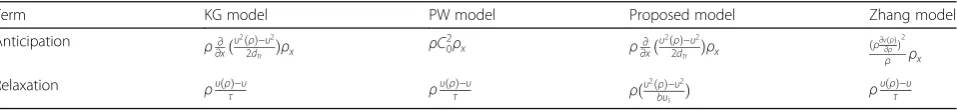
Table 1Traffic model comparison

Term KG model PW model Proposed model Zhang model

Anticipation _ρ∂ ∂xð

υ2_ðρÞ−υ2

2dtr Þρx ρC 2

0ρx ρ_∂∂_xðυ 2_ðρÞ−υ2

2dtr Þρx ðρ

∂vðρÞ ∂ρÞ

2

ρ ρx

Relaxation _ρυðρÞ−υ

τ ρυðρτÞ−υ ρðυ

2_ðρÞ−υ2

bυs Þ ρ

approximates the change in traffic density and flow at the segment boundary. We have that AðGiþ1

2Þ ¼eΛe

−1_,

where Λ is a diagonal matrix of the eigenvalues [λ1,λ2,

⋯,λp] of the Jacobian matrix andeis the corresponding

eigenvector matrix. From [28], the eigenvalues should be positive so that

Δf_iþ1

2¼ej jΛe

−1 _G iþ1−Gi

ð Þ; ð19Þ

where the approximation ΔG= (Gi+ 1−Gi) is used. The

flux at the boundary between segments i and i+ 1 at time_nis then approximated by

fn_iþ1 2 G

n i;Gniþ1

¼1 2 f G

n

i þf Gniþ1

−1 2Δfiþ12;

ð20Þ

where fðGniÞ and fðGniþ1Þ denote the values of the functions of the data variables in road segments i and i+ 1 respectively, at time n. Substituting (19) into (20) gives

fn_iþ1 2 G

n i;Gniþ1

¼1 2 f G

n

i þf Gniþ1

−1 2ej jΛe

−1

Gniþ1−Gni

:

ð21Þ

This approximates the change in density and flow without considering the source.

For the source decomposition of the KG model in (3),

the PW model [15,20] in (12) and the Zhang model in

(14), we have

S1 Gn_i ¼ρn_i υ ρ n i −υni

τ

; ð22Þ

and for the proposed model in (11)

S2 Gn_i ¼ρn_i υ2 _ρn

i − υni 2

bυs

!

: ð23Þ

The updated data variables for the KG, PW, Zhang and proposed models are

Gniþ1¼Gni−

δt δx f

n iþδ

2−f

n iþδx

2

!

þδtSyðGniÞ;y¼1;2: ð24Þ

Both the KG and proposed models have the same ex-pressions on the left-hand side (LHS) as shown in (3)

and (11). Therefore, the Jacobian matrix A(G) is the

same for these models and results in the same eigen-values and eigenvectors, and also average velocity and density. A(G) as well as the corresponding eigenvalues and eigenvectors, average density and velocity for the

KG model were derived in [21]. Assuming the right

hand side (RHS) of the KG and proposed models are in quasilinear form, traffic flow alignment (harmonization)

is not considered so that SyðGÞ ¼ ð00Þ. Then (24) takes

the form

G¼ _ρυρ ;f Gð Þ ¼ f1 f2

¼ ρυ

ρυ ð Þ2

ρ þ υ2_{ð Þρ−υ}2

2dtr ρ 0

B B B @

1 C C C

AandSyð Þ ¼G

0 0 :

ð25Þ

The LHS of (3) and (11) is approximated using the Jacobian matrix ðGÞ ¼∂∂Gf , which is obtained from (25).

The Jacobian matrixAðGÞ ¼_∂∂_Gf from (25) is

A Gð Þ ¼ 0

−υ2_þ υ 2_{ð Þρ −υ}2

2dtr

1

2υ

0 B B @

1 C C

A: ð26Þ

The eigenvalues obtained from (26) inAppendixA are

λ1;2¼υ

ffiffiffiffiffiffiffiffiffiffiffiffiffiffiffiffiffiffiffiffiffiffiffiffiffi

υ2_{ð Þρ −υ}2 2dtr

s

: ð27Þ

These show that when a transition occurs, the velocity changes according to the equilibrium velocity distribu-tion and the average velocity.

For a traffic flow to be strictly hyperbolic, the eigen-vectors must be distinct and real [29]. The eigenvectors corresponding to the eigenvalues in (27) are distinct and real when the equilibrium velocity is greater than the average velocity, i.e.

υ ρ_iþ1 2

>υiþ1 2:

Conversely, the eigenvectors are imaginary when

υ ρ_iþ1 2

<υ_iþ1 2;

so to maintain the hyperbolic property for the proposed model, the absolute value of the numerator under the radical sign in (27) is employed, which gives

λ1;2¼υiþ1 2

ffiffiffiffiffiffiffiffiffiffiffiffiffiffiffiffiffiffiffiffiffiffiffiffiffiffiffiffiffiffiffi

υ2 _ρ iþ1

2

−υ2 iþ1

2

2dtr

v u u t

: ð28Þ

e1;2¼

1

υiþ1 2

ffiffiffiffiffiffiffiffiffiffiffiffiffiffiffiffiffiffiffiffiffiffiffiffiffiffiffiffiffiffiffi

υ2 _ρ iþ1

2

−υ2 iþ1

2

2dtr

v u u t 0

B B B B B B @

1 C C C C C C A

: ð29Þ

The eigenvalues and eigenvectors, average density and

velocity for the PW model were derived in [18]. The

eigenvalues are

λ1;2¼υiþ1

2C0; ð30Þ

where C0 is the velocity constant. This shows that

traffic velocity alignment is at a constant rate C0

during transitions. The corresponding eigenvectors are

e1;2¼ 1

υiþ1 2C0

!

: ð31Þ

The average velocity at the boundary of segments i

andi+ 1 for the KG, PW and proposed models is

υiþ1 2¼

υiþ1

ffiffiffiffiffiffiffiffiffiffiffiffi

ρ_iþ1

p

þυipffiffiffiffiρ_i

ffiffiffiffiffiffiffiffiffiffiffiffi

ρ_iþ1

p

þpffiffiffiffiρ_i : ð32Þ

The average density for these models at the boundary

of segments i and i+ 1 is given by the geometric mean

of the densities in these segments

ρ_iþ1 2¼

ffiffiffiffiffiffiffiffiffiffiffiffi

ρ_iþ1ρi

p _{: ð33Þ}

The eigenvalues for the Zhang model [25] are

λ1¼υiþ1

2; ð34Þ

and

λ2¼υiþ1

2þρvð Þρ ρ; ð35Þ

where the subscriptρpresents the derivative of the equi-librium velocity distribution with respect to density. The corresponding eigenvectors are

e1¼

1

υ_iþ1 2−v ρiþ12

−ρ_iþ1 2v ρiþ12

ρ

0 B @

1 C

A; ð36Þ

e2¼

1

υiþ1 2−v ρiþ12

0 @

1

A_{: ð}37Þ

The average densityρ_iþ1

2of the Zhang model at the

seg-ment boundary is the same as for the KG, PW and pro-posed models given in (33). The average velocity viþ1

2 at

the boundary of segmentsiandi+ 1 for the Zhang model is given inAppendixB.

A. Entropy Fix

Entropy fix is applied to Roe’s technique to smooth any discontinuities at the segment boundaries. The Jacobian matrix AðGiþ1

2Þ is decomposed into its

eigen-values and eigenvectors to approximate the flux in the road segments (21). The Jacobian matrix for the road segments is then replaced with the entropy fix solution given by

ej jΛe−1;

where jΛj ¼ ½^λ1;^λ2;⋯;^λk;⋯;^λn is a diagonal matrix which is a function of the eigenvaluesλkof the Jacobian

matrix, and e is the corresponding eigenvector matrix. The Harten and Hayman entropy fix scheme [30] is employed here so that

^

λk¼ δk^ if j jλk <^δk

λk

j j if j jλk ≥δk^

ð38Þ

with

^

δk ¼ max 0; λiþ1

2−λi; λiþ1−λiþ12

: ð39Þ

This ensures that the ^λ_k are not negative and similar at the segment boundaries. The Jacobian matrix e|Λ|e−1 for the proposed, KG and Zhang models are given in

AppendixC. The corresponding flux is obtained from (21) usingf(Gi) andf(Gi+ 1) and substitutinge|Λ|e−1forAðG_iþ1

2Þ

, the updated data variables,ρandρυ, are then obtained at timenusing (24).

4 Performance results

The performance of the proposed model is evaluated in this section and compared with the KG, PW and Zhang models over a circular road of lengthxM= 100 m. A discontinuous density distributionρ0att= 0 with

peri-odic boundary conditions is employed.ρ0is shown in blue

in the figures. The Greenshields equilibrium velocity dis-tribution given in (13) is used withυm= 34 m/s and max-imum densityρm= 1. The safe distance headway is 28 m, the safe time headway ists= 1.4 s, anddtris 20 m. For the KG and PW models,τ= 1 s. The total simulation time for the proposed and KG models is 30 s. The total simulation time for the PW model is 3 s and for the Zhang model is 4 s. Based onδx= 1 m, the time step for the proposed, KG and Zhang models is chosen as δt= 0.01 s, and the time step for the PW model is chosen asδt= 0.006 s, to satisfy

the CFL condition [31]. The number of time steps and

for the PW model is 500. The number of road steps and time steps for the Zhang model are 100 and 400, respect-ively. The flow regulation parameters considered for the

proposed model areb= 1 and 2. The simulation

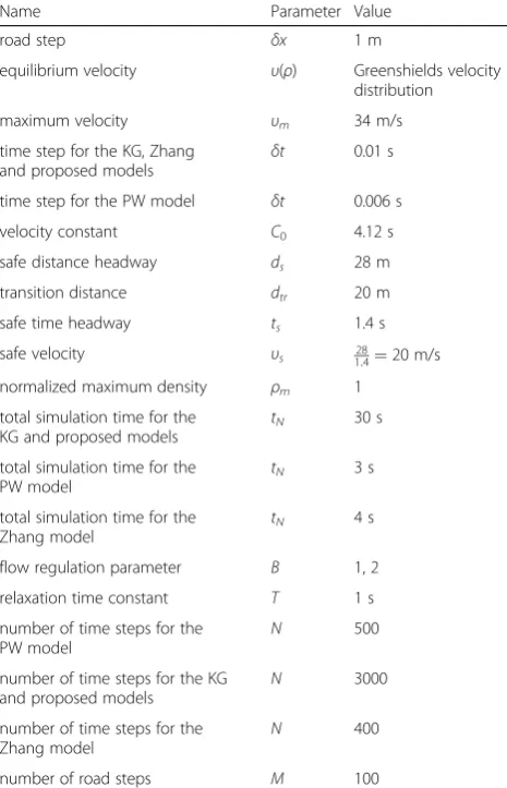
parame-ters are summarized in Table2.

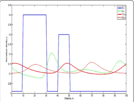
Figure 1 presents the normalized traffic density with

the KG model at four different time instants. This shows that the traffic evolves into two clusters of vehicles. At 5 s the density behavior is slightly oscillatory. However, at 15 s the traffic density beyond 50 m has an almost uniform level of 0.09, and there are two clusters of vehi-cles between 0 and 50 m. The traffic density of these clusters ranges from 0.1 to 0.21. Both clusters span a distance of approximately 20 m. At 30 s, the traffic dens-ity between 0 and 40 m has an almost uniform densdens-ity of 0.09, while beyond 40 m there are two clusters. The clusters still span a distance of about 20 m, so they have just moved over time. The first cluster has a maximum density of 0.25 at 50 m, and the second a maximum density of 0.2 at 78 m.

Figure 2 presents the normalized traffic density with

the proposed model andb= 1 s at four different time in-stants. This shows that with a small value ofb, the traffic becomes quite smooth over time. At 5 s, the variation in traffic density ranges from 0.07 to 0.17, while at 15 s this variation is 0.1 to 0.14, and at 30 s the range is only 0.12 to 0.13. Figure 3 presents the normalized traffic density

behavior with the proposed model and b= 2 s at four

different time instants. There are larger variations in the

density than with b= 1, but smaller than with the KG

model. The traffic evolves into two clusters with a smooth density between them. The variation in density is between 0.09 and 0.16 at 15 s, and between 0.1 and 0. 15 at 30 s.

The traffic velocity behavior with the KG model is given in Fig.4 at four different time instants. The great-est fluctuations in velocity occur at 5 s. At 15 s, the traf-fic has a nearly uniform velocity beyond 50 m of 31 m/s. Table 2Simulation parameters

Name Parameter Value

road step δx 1 m

equilibrium velocity υ(ρ) Greenshields velocity distribution

maximum velocity υm 34 m/s

time step for the KG, Zhang and proposed models

δt 0.01 s

time step for the PW model δt 0.006 s

velocity constant C0 4.12 s

safe distance headway ds 28 m

transition distance dtr 20 m

safe time headway ts 1.4 s

safe velocity υs 28

1:4¼20 m/s

normalized maximum density ρm 1

total simulation time for the

KG and proposed models tN

30 s

total simulation time for the PW model

tN 3 s

total simulation time for the

Zhang model tN

4 s

flow regulation parameter B 1, 2

relaxation time constant Τ 1 s

number of time steps for the PW model

N 500

number of time steps for the KG and proposed models N

3000

number of time steps for the Zhang model

N 400

number of road steps M 100

Fig. 1The KG model density behavior with_τ= 1 s

There are two clusters of vehicles from 0 to 50 m. The velocity in these clusters varies from 27 m/s to 30.2 m/s. At 30 s, between 0 and 40 m the traffic has a near uni-form velocity of 31 m/s, and the two clusters are located beyond 40 m. The first cluster is between 40 and 70 m and has a velocity which varies from 26 to 30.2 m/s, while the second cluster is located between 70 and 90 m and has a velocity which varies from 28 to 30.2 m/s. Comparing the traffic at 15 and 30 s, the velocity in the second cluster increases by 1 m/s, whereas the velocity of the first cluster decreases by 2 m/s.

Figure5presents the velocity behavior at four different

time instants for the proposed model with b= 1. This

corresponds to the density shown in Fig. 2. At 5 s, the variations in velocity are the greatest, ranging from 29 to 31 m/s. At 15 s, this variation is 29.5 to 31.5 m/s, while at 30 s, the difference is less than 1 m/s. These variations

are smaller than with the KG model. Figure 6 presents

the velocity behavior at four different time instants for

the proposed model with b= 2. This corresponds to the

density shown in Fig. 3. The fluctuations in velocity are greatest at 5 s, with a range of 28 to 31 m/s, At 15 s, the range is 29 to 30.5 m/s, while at 30 s it is only 29 to 30. 2 m/s. Thus, the velocity fluctuations are larger than

withb= 1, but smaller than with the KG model.

The traffic flow behavior with the KG model is presented in Fig. 7 at four different time instants. The change in flow follows the changes in density and velocity as it is the product of these two parameters. At 5 s, the flow is more oscillatory, whereas at 15 s the flow evolves into two clusters between 0 and 50 m. The flow in the first cluster varies from 6 veh/s to 3.5 veh/s, while in the second cluster it varies from 6.0 veh/s to 2.8 veh/ s. The flow beyond 50 m aligns to a uniform level of 2.8 Fig. 3The proposed model density behavior withb= 2

Fig. 4The KG model velocity behavior withτ= 1 s

Fig. 5The proposed model velocity behavior withb= 1

veh/s. At 30 s, the two clusters have moved beyond 40 m. The flow in the first cluster now varies from 2.8 to 7.0 veh/s, while in the second cluster it varies from 3. 0 to 5.2 veh/s. The minimum flow between the clusters is 3.0 veh/s at 65 m. In the first 40 m, the flow has an approximately uniform level of 2.8 veh/s.

Figure8 presents the traffic flow behavior at four

dif-ferent time instants with the proposed model andb= 1.

At 5 s, the flow varies from 2.5 to 4.5 veh/s. The max-imum and minmax-imum flows occur at 50 m and 40 m, re-spectively. At 15 s, the flow varies from 3.2 to 4.2 veh/s, which is less than at 5 s. The maximum and minimum flows now occur at 70 m and close to 60 m, respectively. At 30 s, the flow is only in the range 3.5 to 4.0 veh/s,

and the maximum flow occurs at 40 m. Figure 9

pre-sents the corresponding traffic flow behavior with the

proposed model andb= 2. The behavior is more

oscilla-tory at 5 s, and the flow varies from 2.5 to 6.0 veh/s, which is greater than withb= 1. At 15 s, the flow varies from 3.0 to 4.5 veh/s, and it is almost the same at 30 s. However, the locations of the maximum and minimum traffic flows are different.

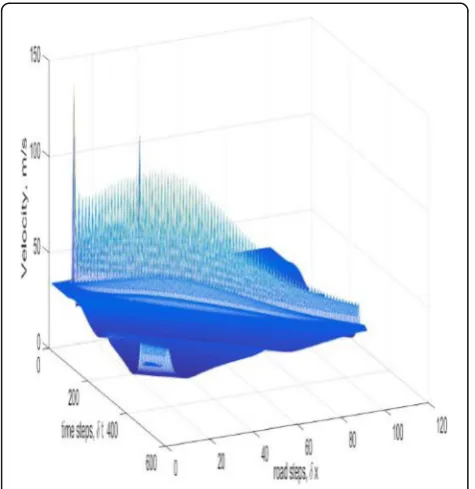
The velocity behavior on the road over a time span of

3 s with the PW model is given in Fig. 10. This shows

that the variations in velocity increase over time. In

par-ticular, the velocity exceeds 300 m/s and goes below −

200 m/s, even though the maximum and minimum vel-ocities are 34 m/s and 0 m/s, respectively. Thus the PW model produces unrealistic behavior. Further, the vel-ocity is more oscillatory with the PW model than with the proposed model. The traffic velocity behavior with the Zhang model over a time span of 4 s is shown in Fig. Fig. 7The KG model flow withτ= 1 s

Fig. 8The proposed model flow withb= 1

Fig. 9The proposed model flow withb= 2

11. The traffic velocity goes up to 140 m/s, which is well above the maximum velocity 34 m/s. Over time, the variations in velocity decrease. The velocity is more oscillatory than the proposed model and is unrealistic. The results in this section show that the flow

regula-tion parameterbin the proposed model can be used to

adjust traffic oscillations and cluster behavior. For

smaller values of b, traffic becomes more uniform.

Thus, unrealistic oscillations can be eliminated with this parameter, and traffic behavior can be properly characterized.

5 Conclusion

In this paper, a new model was proposed to

characterize the physiological and psychological

response of drivers to changes in the traffic flow. For a slow response, the traffic becomes clustered, while for a fast response the traffic flow is more uniform. A regulation parameter was introduced to characterize driver response to forward conditions. This allows for more realistic traffic characterization than with other models in the literature. With smaller values of the regulation parameter in the proposed model, changes in velocity are reduced and the traffic flow becomes smooth. Pollution emissions increase with changes in velocity, in particular carbon monoxide, nitric oxide and hydrocarbon emissions are greater at higher vel-ocities. However, velocities between 16.7 m/s and 22. 2 m/s result in reduced fuel consumption and

pollution [32]. Variations in velocity can be reduced

with the regulation parameter b in autonomous

vehi-cles to reduce fuel consumption and pollution. The proposed model can help in analyzing the behavior of autonomous vehicles. This will lead to more accurate results which can be employed to reduce fuel con-sumption and pollution.

6 Appendix

A:Eigenvalues λ1;2 ðEigenvaluesÞ

A Gð Þ ¼ 0

−υ2_þ υ 2_{ð Þρ −υ}2

2_dtr

1

2υ

0 B B @

1 C C

A: ð40Þ

At the road segment boundaries, the eigenvalues λi of the Jacobian matrix are required to obtain the flux in (21), and are obtained as the solution of

A Gð Þ−λI

j j ¼ −λ

−υ2þ υ 2_{ð Þρ −υ}2

2dtr

1

2υ−λ

¼0; ð41Þ

which gives

λ2₋

2υλþυ2− υ 2_{ð Þρ −υ}2

2dtr

¼0: ð42Þ

The eigenvalues are then

λ1;2¼

2υ

ffiffiffiffiffiffiffiffiffiffiffiffiffiffiffiffiffiffiffiffiffiffiffiffiffiffiffiffiffiffiffiffiffiffiffiffiffiffiffiffiffiffiffiffiffiffiffiffiffiffi

4υ2_{−4 υ}2₋ υ

2_{ð Þρ −υ}2

2dtr

s

2

¼υ

ffiffiffiffiffiffiffiffiffiffiffiffiffiffiffiffiffiffiffiffiffiffiffiffiffi

υ2_{ð Þρ−υ}2

2_dtr

s

:

B. Zhang Model Average Velocity

Using Roe scheme, the average velocity at the boundary of segmentsiandi+ 1 for the Zhang model is

viþ1 2¼

−bþpffiffiffiffiffiffiffiffiffiffiffiffiffiffiffib2−4ac

2_a ð43Þ

where

b¼− ρ_iþ1 2v ρiþ12

−ρ_i−1 2v ρi−12

h i

−vð Þρ ρ_iþ1

2−ρi−12

−2ρ_iþ1 2 viþ

1 2−v ρiþ12

þ2ρ_i−1 2 vi−

1 2−v ρi−12

;

c¼vð Þρ ρiþ1 2v ρiþ

1 2

−ρ_i−1 2v ρi−

1 2

h i

þvð Þρ ρ_iþ1

2 viþ 1 2−v ρiþ12

−ρ_i−1 2 vi−

1 2−v ρi−12

− viþ12−v ρiþ12

ρiþ1 2

2

ρ_iþ1 2

þv ρiþ1 2

viþ1 2−v ρiþ12

ρiþ1 2 0 B @ 1 C A

þ vi−12−v ρi−12

ρ_i−1 2

2

ρ_i−1 2

þv ρi−1 2

vi−1 2−v ρi−12

ρi−1 2 0 B @ 1 C A:

C. Jacobian Matrix for Entropy Fix

The Jacobian matrix e|Λ|e−1 for both the proposed and KG models is

ej jΛe−1¼ 1

υiþ1 2þ

ffiffiffiffiffiffiffiffiffiffiffiffiffiffiffiffiffiffiffiffiffiffiffiffiffiffiffiffiffiffiffi

υ2 _ρ iþ1

2

−υ2 iþ1

2

2dtr

v u u t

1

υiþ1 2−

ffiffiffiffiffiffiffiffiffiffiffiffiffiffiffiffiffiffiffiffiffiffiffiffiffiffiffiffiffiffiffi

υ2 _ρ iþ1

2

−υ2 iþ1

2

2dtr

v u u t 0 B B B B B B @ 1 C C C C C C A

υiþ1 2þ

ffiffiffiffiffiffiffiffiffiffiffiffiffiffiffiffiffiffiffiffiffiffiffiffiffiffiffiffiffiffiffi

υ2 _ρ iþ1

2

−υ2 iþ1

2

2dtr

v u u t 0 0

υiþ1 2−

ffiffiffiffiffiffiffiffiffiffiffiffiffiffiffiffiffiffiffiffiffiffiffiffiffiffiffiffiffiffiffi

υ2 _ρ iþ1

2

−υ2 iþ1

2

2dtr

v u u t 0 B B B B B B B B B @ 1 C C C C C C C C C A υiþ1

2−

ffiffiffiffiffiffiffiffiffiffiffiffiffiffiffiffiffiffiffiffiffiffiffiffiffiffiffiffiffiffiffi

υ2 _ρ

iþ1 2

−υ2

iþ1 2

2dtr v u u t

−υiþ1 2−

ffiffiffiffiffiffiffiffiffiffiffiffiffiffiffiffiffiffiffiffiffiffiffiffiffiffiffiffiffiffiffi

υ2 _ρ

iþ1 2

−υ2

iþ1 2

2dtr v u u t −1 1 0 B B B B B B @ 1 C C C C C C A −1 2 ffiffiffiffiffiffiffiffiffiffiffiffiffiffiffiffiffiffiffiffiffiffiffiffiffiffiffiffiffiffiffi

υ2 _ρ iþ1

2

−υ2 iþ1

2

2dtr

v u u t

;

The Jacobian matrix for the PW model is

ej jΛe−1¼ _υ 1

iþ1 2þC0

1

υ_iþ1 2−C0

!

υiþ1 2þC0

0

0

υiþ1 2−C0

0 B @ 1 C

A υiþ1 2−C0

−υ_iþ1 2−C0

−1 1

!

−1 2C0;

and the Jacobian matrix for the Zhang model is

ej jΛe−1_¼ 1

υiþ1 2−v ρiþ12

−ρiþ1 2v ρiþ12

ρ

1

υiþ1 2−v ρiþ12

0 B @ 1 C A

υiþ1 2−v ρiþ12

−ρ_iþ1 2v ρiþ12

ρ 0 0

υiþ1 2−v ρiþ12

0 B B @ 1 C C A

υiþ12−v ρiþ12

−υiþ1

2þv ρiþ12

þv ρiþ1 2 ρ −1 1 0 B @ 1 C A 1

ρiþ1 2v ρiþ12

ρ ;

Publisher’s Note

Springer Nature remains neutral with regard to jurisdictional claims in published maps and institutional affiliations.

Author details

1_{Electrical Engineering Department, University of Engineering and} Technology, Peshawar, Pakistan.2Department of Electrical and Computer Engineering, University of Victoria, PO Box 1700, STN CSC, Victoria, BC V8W 2Y2, Canada.

Received: 12 September 2017 Accepted: 5 April 2018

References

1. Davoodi N, Soheili AR, Hashemi SM (2016) A macro-model for traffic flow with consideration of driver's reaction time and distance. Nonlinear Dynam 83:1621_–1628

2. Del Castillo JM, Pintado P, Benitez FG (1994) The reaction time of drivers and the stability of traffic flow. Transpn Res B 28:35–60

3. Jamshidnejad A, Papamichail I, Papageorgiou M, Schutter B (2017) A mesoscopic integrated urban traffic flow emission model. Transpn Res C 75:45–83

4. Newell GF (1961) Nonlinear effects in the dynamics of car following. Operations Res 9:209–229

5. Berthaume AL (2015) Microscopic modeling of driver behavior based on modifying field theory for work zone application. Dissertation, University of Massachusetts Amherst

6. Chandler RE, Herman R, Montroll EW (1958) Traffic dynamics: studies in car following. Operations Res 6:165_–184

7. Gazis DC, Herman R, Rothery RW (1961) Non-linear follow the leader models of traffic flow. Operations Res 9:545–567

8. Gipps PG (1981) A behavioral car following model for computer simulation. Transpn Res B 15:105_–111

9. Wiedemann R (1974) Simulation des straßenverkehrsflusses. Schriftenreihe des IfV, Institut für Verkehrswesen, Universität Karlsruhe

10. Higgs B, Abbas M M, Medina A (2011) Analysis of the Wiedemann car following model over different speeds using naturalistic data. Proc Int Conf on Road Safety and Simulation

11. Romoser MRE, Fisher DL (2009) The effect of active versus passive training strategies on improving older drivers’scanning in intersections. Hum Factors 51:652_–668

12. Pollatsek A, Romoser MRE, Fisher DL (2012) Identifying and remediating failures of selective attention in older drivers. Curr Dir Psychol Sci 21:3–7 13. Liu Z, Zhao Y, Wang P (2012) Road traffic safety engineering. Higher

Education Press, Beijing

14. Mourant RR, Rockwell TH (1972) Strategies of visual search by novice and experienced drivers. Hum Factors 14:325–335

15. Payne HJ (1971) Models of freeway traffic and control. Simulation Council Proc 1:51_–61

17. Daganzo CF (1995) Requiem for second-order fluid approximations of traffic flow. Transpn Res B 29:277_–286

18. Balogun SK, Shenge NA, Oladipo SE (2012) Psychosocial factors influencing aggressive driving among commercial and private automobile drivers in Lagos metropolis. Social Sci J 49:83–89

19. Zhang HM (1998) A theory of non-equilibrium traffic flow. Transpn Res B 32:485–498

20. Zhang HM (2002) A non-equilibrium traffic model devoid of gas-like behaviour. Transpn Res B 36:275–290

21. Khan Z (2016) Traffic flow modelling for intelligent transportation systems. Dissertation, University of Victoria

22. Emerson JL, Johnson AM, Dawson JD, Uc EY, Anderson SW, Rizzo M (2012) Predictors of driving outcomes in advancing age. Psychol Aging 27:550–559 23. Hindmarch I, Kerr JS, Sherwood N (1991) The effects of alcohol and other

drugs on psychomotor performance and cognitive function. Alcohol Alcohol 26:71–79

24. Guo M, Li S, Wang L, Chai M, Chen F, Wei Y (2016) Research on the relationship between reaction ability and mental state for online assessment of driving fatigue. Int J Environ Res Public Health 13:1174–1189 25. Morgan JV (2002) Numerical methods for macroscopic traffic models.

Dissertation, University of Reading

26. Greenshields BD (1935) A study in highway capacity. Proc Highway Res Board 14:448–477

27. Roe PL (1981) Approximate Riemann solvers, parameter vectors, and difference schemes. J Comput Phys 43:357–372

28. Leer BV, Thomas JL, Roe PL, Newsome RW (1987) A comparison of numerical flux formulas for the Euler and Navier-stokes equations. Proc American Inst Aeronautics and Astronautics Computational Fluid Dynamics Conf 87-1104:36–41

29. Toro EF (2009) Riemann solvers and numerical methods for fluid dynamics. Springer, Berlin

30. Harten A, Hayman JM (1983) Self adjusting grid methods for one-dimensional hyperbolic conservation laws. J Comput Phys 50:253–269 31. LeVeque RJ (1992) Numerical methods for conservation Laws. Springer,

Birkhäuser, Basel