Conditional Relationship Between Beta and Return in the US Stock Market

(1)

http://Business.ExpertJournals.com

46

Conditional Relationship Between Beta and

Return in the US Stock Market

Bing XIAO

*

Université d’Auvergne, France

According to the CAPM, risk is measured by the beta, and the relation between required expected return and beta is linear. This paper examines the conditional relationship between beta and return in the US stock market. The conditional covariances and variances used to estimate beta are modeled as an ARCH process. The beta return relationship is tested upon the sign of the excess market return. The implication of the sign of the excess market return follows Morelli (2011). This study shows the importance of recognizing the sign of the excess market return when testing the beta-return relationship. The approach also allows us to distinguish the size effect and the effect of economic cycles.

Keywords: Conditional beta, Market risk premium, ARCH models, US stock market

JEL Classification: C52, G1, G10, G12

1. Introduction

The CAPM is widely viewed as one of major contributions of academic research to financial managers. But the robustness of the size effect and the absence of a relation between beta and average return are so contrary to the CAPM that the consensus is that the static CAPM is unable to explain the cross-section of average returns on stocks (see Fama and French, 1992).

This paper examines the role of beta in explaining security returns in the US stock market over the period of October 2000 to June 2014. In this paper, the author adopts the dynamic conditional beta approach proposed by Morelli (2011). We use univariate GARCH models to estimate the dynamic of the volatility of error terms, and a dynamic of the dependence structure between the innovations. The beta is estimated as the ratio of the conditional covariance between the residuals from an autoregressive model for each index return and market return, and the conditional variance of the residuals from an autoregressive model for the market return. Modeling both components of beta (the covariance and variance) as an ARCH/GARCH process allows conditional information to be incorporated into the model (see Morelli 2011).

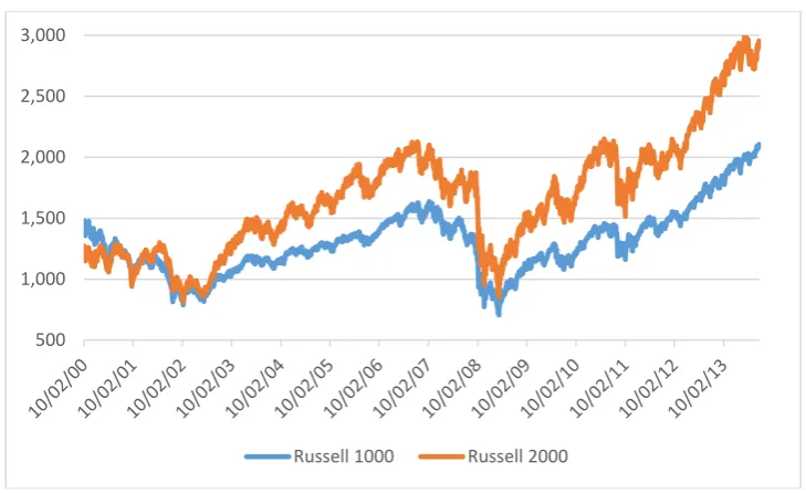
The empirical investigation is based on the Russell 3000 index which consists of 3,000 stocks. It subdivides into large and small cap indexes. The large cap index is the Russell 1000, which consists of the top 1,000 companies, give or take a few. The small cap index is the Russell 2000, which includes all the rest of the Russell 3000. The large-cap Russell 1000 had a market-cap range of $1.35 billion to $540 billion, with a

*_{Corresponding Author:}

Bing Xiao, CRCGM EA 38 49, Université d’Auvergne, Auvergne, France Article History:

Received 5 March 2016 | Accepted 28 March 2016 | Available Online 7 April 2016 Cite Reference:

(2)

47

median of $5.2 billion. The small-cap Russell 2000 had a range of $101 million to $2.61 billion, with a median of $460 million. The testing period is also split into two subperiods running form October 2, 2000 to January 25 2007 and January 25, 2007 to June 24, 2014. This allows us to calibrate the model with data during two economic cycles.

The rest of the paper is organized as follows. Section 2 details the reviews of literature. Section 3 presents the methodology and the data. Section 4 discusses our estimates of conditional beta. Section 5 concludes the paper.

2. Literature Review

The Sharpe-Lintner-Black Capital Asset Pricing Model (CAPM) is a capital asset pricing model that financial managers use most often for assessing the risk. According to the CAPM, the risk is measured by the beta, and the relation between required expected return and beta is linear. Many subsequent studies failed to find a risk-return relationship.

Banz (1981) was one of the first researchers to study the influence of market capitalisation on security returns. He demonstrated that small cap securities generated greater returns than those of large capitalisation and attributed this overperformance of small caps to the remuneration of an additional risk factor.

The size effect also poses a problem with regards to the validity of the Capital Asset Pricing Model (CAPM), validity according to which which the expected yield of securities depends on the systematic risk level (the beta). According to behavioural finance researchers, size effect is proof of the irrationality of individuals. On the other hand, researchers who support the concept of rationality suggest that size effect can be attributed to risk factors other than the market.To reconcile the size effect with the CAPM, Fama and French (1992, 1993) proposed incorporating additional risk factors into it, as the beta was no longer the sole source of risk. Fama and French suggested that the higher than expected returns of value stocks and small caps offset the additional risk inherent in these securities for shareholders. In fact, value stocks and small caps are susceptible to being financially weakened in the event of an economic crisis.

The CAPM model is based upon expectation, and it is tested using realized returns with the assumption that realized returns accurately reflect, and thus can proxy for. The positive relationship between beta and the expected returns implies that the expected return on the market must always exceed the risk-free rate and the expected market risk premium is positive (see Morelli 2011). Using realized data, the realized market risk premium may be negative (see Pettengill et al. 1995). They claimed that there is a probability that the return on the market will at times be less than the risk-fee rate. If this was not the case, no rational investor would ever invest in risk-free assets. Pettengill et al. (1995) infer that when the realized return on the market exceeds the risk-free rate (up markets) there exists a positive relationship between beta and returns, and when the realized market return is negative (down markets) the beta return relationship should be negative. Morelli (2011) confirmed this assumption by examining the role of beta in explaining security returns in the UK stock market.

The CAPM was derived by examining the behavior of investor in a hypothetical model-economy in which they live for one period. In the real world investors live for many periods. One of the assumptions is that the betas of the assets remain constant over time. Jagannathan and Wang (1996) suggested that the assumption is not reasonable since the relative risk of a firm’s cash flow vary over the business cycle. During a recession, for example, financial leverage of firms in relatively poor shape may increase sharply relative to other firms, causing their stock betas to rise. Hence, betas and expected returns depend on the nature of the information available at any given point in time and vary over time.

3. Data and Methodology

3.1.Data

(3)

48

Figure 1. Russell 1000 and Russell 2000 index (Daily, 2000 – 2014)

The summary statistics for the Russell 1000, Russell 2000 and Russell 3000 index (Table A1 in the Appendix) reveals a positive skewness, and a positive kurtosis. Russell index are non-normal at the confidence interval of 99%. So, it is mandated to convert the Russell index series into the return series.

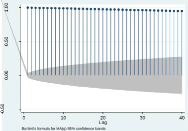
By observing the plotted autocorrelation and partial autocorrelation of the Russell 3000 index we find that the series is nonstationary (Figures A1 and A2 in the Appendix). This is confirmed when we apply both the Dickey-Fuller test and the Phillips-Perron test (Table A2, A3 in the Appendix), so in this case we cannot use the ARCH model for modelling volatility.

In general, the movements of the stock indices series are non-stationary and not appropriate for the study purpose. So, it is mandated to convert the daily price into the return series. The series of Russell index are transformed into returns by using the following equation:

𝑅𝑡 = ( 𝑃_𝑡

𝑃_𝑡−1) − 1 (1)

Where,

Rt = the rate of return at time t

Pt = the price at time t

Pt-1 = the price just prior to the time t

The summary of statistics on returns are found in Table 1. This table also shows that that Russell 3000 index has an average daily return of 0.0001833 percent and a standard deviation of 0.01264. In accordance with most financial time series, the skewness coefficient, -0.03531, has a negative sign. Therefore, these characteristics of data can be accounted for by using the ARCH family of models. And so, when modeling such a series the series must be stationary. Because of this, the Dickey-Fuller test is applied to the returns series (Table A4 in the Appendix). In the results of this test we can observe that the series is indeed stationary. The Phillips-Perron test confirms that the series is stationary (Table A5 in the Appendix).

Table 1. Summary statistics for returns

Obs Mean Std. Dev. Min Max Skewness Kurtosis

Russell1000 3581 0.000178 0.0002139 0.0911 0.1167 0.004622 8.6750

Russell2000 3581 0.000356 0.0006237 -0.1185 0.09265 0.123882 4.6165

Russell3000 3581 0.000190 0.0002162 0.0928 0.1147 0.029767 8.1954

ADF test as well as PP test are used to get confirmation regarding whether the return series is stationary or not. The values of ADF test statistic, -68.545, is less than its test critical value, -3.410, at 5%, level of significance which implies that the crude oil price return series is stationary. The findings of the PP test also confirms that return series is stationary, since the values of PP test statistic is less than its test critical value.

500 1,000 1,500 2,000 2,500 3,000

(4)

49

The plotted autocorrelation and partial autocorrelation of squared returns indicate dependence, and therefore suggest time-varying volatility (Figures A3 and A4 in the Appendix). From this data we can deduce that the series are time-dependent.

3.2.Specification of the Models Used in This Study

3.2.1. ARCH(q) Model and GARCH(p, q) Model

Autoregressive conditional heteroskedasticity (ARCH) models are used when the error terms will have a characteristic size or variance (Engle 1982). The ARCH models assume the variance of the current error term to be a function of the actual sizes of the previous time period’s error terms. The ARCH model is a non-linear model which does not assume the variance is constant. The error terms are split into a stochastic piece and a time dependent standard deviation:

𝜖𝑡 = 𝜎𝑡𝑧𝑡 (2)

The random variable is a white noise process, the series σ2

t is modelled by:

𝜎𝑡2 = 𝑎0+ 𝑎1𝜖𝑡−12 + ⋯ + 𝑎𝑞𝜀𝑡−𝑞2 = 𝑎0+ ∑𝑞𝑖=1𝑎𝑖𝜀𝑡−𝑖2 (3) Where a0 > 0 and ai > 0.

The GARCH model is a generalized ARCH model, developed by Bollerslev (1986) and Taylor (1986) independently. The GARCH model is a solution to avoid problems with negative variance parameter estimates. A fixed lag structure is imposed. The GARCH (p, q) model (where p is the order of the GARCH terms σ2_and

q is the order of the ARCH terms ε2_.

𝜎𝑡2= 𝑤 + 𝑎1𝜖𝑡−12 + ⋯ + 𝑎𝑞𝜀𝑡−𝑞2 + 𝛽1𝜎𝑡−12 + ⋯ + 𝛽𝑝= 𝑤 + ∑𝑞𝑖=1𝑎𝑖𝜀𝑡−𝑖2 + ∑𝑝𝑖=1𝛽𝑖𝜎𝑡−𝑖2 (4) The form of GARCH (1,1) is given below:

𝜎_𝑡2_{= 𝑎}

0+ 𝑎1𝜀𝑡−12 + 𝛽𝜎𝑡−12 (5)

3.2.2. The Conditional Relationship between Risk and Return

The conditional version of the CAPM can be shown as follows:

𝐸(𝑟𝑖𝑡|∅𝑡−1) = 𝛽𝑖|∅𝑡−1(𝐸(𝑟𝑀𝑡|∅𝑡−1)) (6) Where 𝑟𝑖𝑡 is the excess return for security i and rMt is the excess return on the market portfolio,

E (. | ∅t-1) is expectation conditional on the information set ∅ available at time t-1. βi is the beta coefficient of

security i, the measure of systematic risk given by the following expression (see Morelli 2011):

𝛽𝑖|∅𝑡−1 = 𝑐𝑜𝑣(𝑟𝑖𝑡, 𝑟𝑀𝑡|∅𝑡−1) 𝑣𝑎𝑟(𝑟⁄ 𝑀𝑡|∅𝑡−1) (7) Tests of the conditional relationship between beta and returns depend upon the information set ∅

available. Different tests can be conducted dependent upon how the information set ∅ is defined. In this article, the ∅ represents econometric information.

The return on equity i and the market can be modeled as an autoregressive process as given by :

𝑟𝑖𝑡 = 𝑎0+ ∑𝑛𝑗=1𝑎𝑗𝑟𝑖𝑡−𝑗+ 𝜀𝑖𝑡 (8)

𝑟𝑀𝑡 = 𝑎0+ ∑𝑛𝑗=1𝑎𝑗𝑟𝑀𝑡−𝑗+ 𝜀𝑀𝑡 (9)

These two equations can be decomposed into the expected and unexpected components as follows:

𝑟𝑖𝑡 = 𝐸(𝑟𝑖𝑡|∅𝑡−1) + 𝜀𝑖𝑡 (10)

𝑟𝑀𝑡 = 𝐸(𝑟𝑀𝑡|∅𝑡−1) + 𝜀𝑀𝑡 (11)

The disturbance terms εit, εMt can be decomposed, and the expectation part of the equation represents

the conditional covariance between rit, rMt and the conditional variance of rMt respectively. So, the risk

measurement beta can be expressed as follows:

𝛽𝑖|∅𝑡−1 = 𝐸(𝑟𝑖𝑡, 𝑟𝑀𝑡|∅𝑡−1) 𝐸(𝑟⁄ 𝑀𝑡|∅𝑡−1)= 𝑐𝑜𝑣(𝑟𝑖𝑡, 𝑟𝑀𝑡|∅𝑡−1) 𝑣𝑎𝑟(𝑟⁄ 𝑀𝑡|∅𝑡−1) (12) The expected return on an equity is dependent upon time varying risk, where the conditional information is incorporated by modeling the components of risk as ARCH and GARCH processes.

𝐸(𝑟𝑖𝑡|∅𝑡−1) = (𝛽𝑖|∅𝑡−1)[𝐸(𝑟𝑀𝑡|∅𝑡−1)] (13) In order to proceed with the estimation of beta by equation (12), it is necessary for the expectations appearing in both the numerator and the denominator (see Morelli 2011). Each of the expectations E (εit εMt)

and E (ε2

Mt) (var (rMt|∅t-1)) will be a function of the econometric information available at time t-1. rit, rMt can

be represented by an autoregressive process. And for both components of conditional beta, E (εit εMt) and E

(ε2

Mt), they could follow an ARCH or GARCH process, a model where the conditional variances and

covariances are allowed to change over time. All the heteroskedastic models are adopted in the estimation process with the best fit model being the one selected.

(5)

50

𝑟𝑖= 𝑎0+ 𝛾1𝛽𝑖+ 𝜀𝑖 (14)

Where a0 should equal zero and γ1 is the market risk premium. A positive γ1 implies that the beta is a

significant risk measure. We suppose the relationship between beta, returns conditional and the excess market return. We use a model with a dummy variable in the cross-sectional. The dummy variable separated the positive and negative excess market returns. The equation is shown as follows (see Pettengill et al. 1995):

𝑟𝑖= 𝑎0+ 𝜃𝛾1+𝛽𝑖+ (1 − 𝜃)𝛾1−𝛽𝑖+ 𝜀𝑖 (15) Where θ = 1 if rMt > 0 and 0 if rMt < 0. The positive and negative symbol of γ mean a positive and

negative excess market return. The dummy variable allows us to examine the negative market risk premium. The a0 should equal 0 and the γ should be significant. Morelli (2011) pointed that the methodology of Pettengill

et al. (1995) is not a test of CAPM, but a test of the significance of beta, and they focused on the relationship between beta and realized returns and not expected returns.

4. Empirical Findings (Analysis and Results)

We find a significant autocorrelation at differing lags are detected for the Russell 1000 and Russell 3000 index, reducing in significance as the lag period increases (Appendix A1, A2). An autoregressive process is required to produce an uncorrelated sequence from the return series. The author found an ARMA(1,1) process for the two index. The residual series is strict white noise and shows no significant autocorrelation (Appendix A11, 12, 15, 16). Beta estimation requires the conditional variance and the covariance, both of which are modeled as an ARCH process.

Having estimated both the conditional variance and the conditional covariance, beta is then estimated in accordance with equation (12). Table (2) reports the results from the cross-sectional regression as given by equation (14), showing the average risk premium of Russell 1000 over the total time period, γ= -0.04017, and also for the two sub-periods, γ=0.01919 and γ=-0.2049.

Table 2. The relationship between beta and returns

October 2000 to June 2014

October 2000 to January 2007

January 2007 to June 2014

α (Russell 1000) 0.04024

(0.373)

-0.01915 (0.851)

0.2039 (0.166)

γ (Russell 1000) -0.04017

(0.375)

0.01919 (0.851)

-0.2049 (0.167)

α (Russell 2000) -0.00237

(0.621)

0.00011 (0.991)

-0.01865 (0.216)

γ (Russell 2000) 0.002671

(0.568)

0.00025 (0.981)

0.01783 (0.207)

Note: The table reports the time-series coefficients (risk premiums) over the testing periods. The p-values is shown in parentheses.

The positive risk premium implies an upward sloping risk-return relationship (see Morelli 2011). The risk premium in our study is not statistically significant, so the hypothesis which γ≠0 is rejected, and beta does not play a significant role in explaining security returns. Such findings are consistent with studies on the US markets by Davis (1994) and Fama and French (1992) and the study on the UK market by Morelli (2011). Morelli (2011) noted that the insignificant beta can be explained by the aggregation of data during periods when excess market return is both positive and negative.

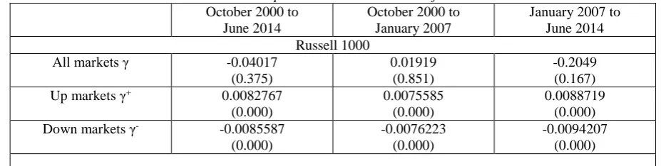
Table 3. The relationship between beta and returns for Russell index

October 2000 to June 2014

October 2000 to January 2007

January 2007 to June 2014 Russell 1000

All markets γ -0.04017

(0.375)

0.01919 (0.851)

-0.2049 (0.167)

Up markets γ+ _0.0082767

(0.000)

0.0075585 (0.000)

0.0088719 (0.000)

Down markets γ- _-0.0085587

(0.000)

-0.0076223 (0.000)

(6)

51 Russell 2000

All markets γ 0.002671

(0.568)

0.00025 (0.981)

0.01783 (0.207)

Up markets γ+ _0.0100167

(0.000)

0.0092839 (0.000)

0.0105116 (0.000)

Down markets γ- _-0.010144

(0.000)

-0.0088223 (0.000)

-0.0111427 (0.000)

Note: The table reports the time-series coefficients (risk premiums) in all markets and up and down markets, the t-statistics is shown in parentheses.

Table 3 reports the results from testing the beta-return relationship conditional on the sign of the excess market return (Eq. (15)), reporting the average risk premium in both up and down markets. The results from the cross-sectional regression show a significant positive relationship between beta and returns during up markets, and a significant negative relationship between beta and returns. The null hypothesis of no beta-return relationship is rejected. The mean value of the regression coefficient γ+_{for the Russell 1000 index is}

0.0082767, and the mean value of the regression coefficient γ+_{for the Russell 2000 is 0.0100167. Such finding}

implies that during up markets high beta portfolios exhibit higher returns than low beta portfolios.

The mean value of the regression coefficient γ-_{for the Russell 1000 index is -0.0085587, and the mean}

value of the regression coefficient γ-_{for the Russell 2000 is -0.010144. Such findings imply that during down}

markets high beta portfolios earn lower returns than low beta portfolios. This results conform to the findings of Morelli (2011), which suggest that beta risk is rewarded in up markets for losses incurred in down markets. This significant beta-return relationship holds across the total time period and also across both subperiods.

5. Conclusion

This paper contributes to the existing literature regarding the role of beta in explaining security returns by incorporating ARCH models to estimate time varying betas. The empirical result show that when the sign of the excess market return is ignored beta is found to be an insignificant risk factor. During periods when the excess market return is positive, a significant positive relationship is found between beta and returns. And during periods when the excess market return is negative, a significant negative relationship is found between beta and returns. This finding confirms the hypothesis of Pettengill et al. (1995) and Morelli (2011). However, the beta is found to be an insignificant risk measurement in the absence of recognition of the sign of the excess market return. This being said, in spite of the lack of empirical support, the CAPM is still the preferred model for managerial finance courses, because the empirical support for other asset-pricing models is no better. It is important to investigate the relationship between conditional beta and the security returns in the equity markets of other countries.

References

Banz R.W., 1981. The Relationship between return and market value of common stocks. Journal of Financial Economics, 9 (1), pp.3-18.

Black, F., Jensen, M.C. and Scholes, M., 1972. The capital asset pricing model: some empirical tests.’ In: Jensen, M.C. (Ed.), Studies in the Theory of Capital Markets, Praeger, NY, pp.79–124.

Bollerslev, T., 1986. Generalized autoregressive conditional heteroscedasticity. Journal of Econometrics, 31, pp.307–327, [online] Available online at: http://dx.doi.org/10.1016/0304-4076(86)90063-1

Engle, R.F., 1982. Autoregressive conditional heteroscedasticity with estimates of the variance of the United Kingdom Inflation. Econometrica, 50, pp.987–1007. [online] Available online at: http://dx.doi.org/10.2307/1912773

Engle, R.F., Jondeau E. and Rockinger M., 2012. Dynamic Conditional Beta and Systemic Risk in Europe. [online] Available online at:

http://www.stern.nyu.edu/sites/default/files/assets/documents/con_037459.pdf

Engle, R.F., Bali, T.G. and Tang, Y., 2013. Dynamic conditional beta is alive and well in the cross section of

daily stock returns. Working paper 1305. [online] Available online at:

http://papers.ssrn.com/sol3/papers.cfm?abstract_id=2089636&rec=1&srcabs=2078295&alg=1&pos =10

(7)

52

Fama, E. F. and French, K. R., 1995. Size and book to market factors in earnings and returns. The Journal of Finance, 50 (1), pp.131-155.

Jagannathan, R. and Wang, Z., 1996. The conditional CAPM and the cross-section of expected returns’.

Journal of Finance, 51, pp.3–53, [online] Available online at: http://dx.doi.org/10.1111/j.1540-6261.1996.tb05201.x

Lewellen, J. and Nagel, S., 2006. The Conditional CAPM does not explain asset pricing anomalies. Journal of

Financial Economics, 82(2), pp.289-314. [online] Available online at:

http://dx.doi.org/10.1016/j.jfineco.2005.05.012

Lintner, J., 1965. The valuation of risky assets and the selection of risky investments in stock portfolios and capital budgets. Review of Economics and Statistics, 47, pp.13–37, [online] Available online at: http://dx.doi.org/10.2307/1924119

Morelli, D.A., 2007. Conditional relationship between beta and return in the UK stock market. Journal of Multinational Financial Management, 17, pp.257–272, [online] Available online at: http://dx.doi.org/10.1016/j.mulfin.2006.12.003

Morelli, D.A., 2011. Joint conditionality in testing the beta-return relationship: Evidence based on the UK stock market. Journal of International Financial Markets, Institutions & Money, 21, pp.1-13, [online] Available online at: http://dx.doi.org/10.1016/j.intfin.2010.05.001

Musaddiq, T., 2012. ‘Modeling and Forecasting the Volatility of Oil Futures Using the ARCH Family Models.

The Lahore Journal of Business, 1(1), pp.79–108.

Pettengill, G., Sundaram, S. and Mathur, I., 1995. The conditional relation between beta and returns. Journal of Financial and Quantitative Analysis, 30, pp.101–116. [online] Available online at: http://dx.doi.org/10.2307/2331255

(8)

53 -0 .5 0 0 .0 0 0 .5 0 1 .0 0 Au to co rre la ti o n s o f ru s se ll3 0 0 0

0 10 20 30 40

Lag

Bartlett's formula for MA(q) 95% confidence bands

0 .0 0 0 .2 0 0 .4 0 0 .6 0 0 .8 0 1 .0 0 Pa rt ia l a u to co rre la ti o n s o f ru sse ll3 0 0 0

0 10 20 30 40

Lag

95% Confidence bands [se = 1/sqrt(n)]

-0 .1 0 0 .0 0 0 .1 0 0 .2 0 0 .3 0 0 .4 0 Au to co rre la ti o n s o f r2

0 10 20 30 40

Lag

-0 .2 0 0 .0 0 0 .2 0 0 .4 0 Pa rt ia l a u to co rre la ti o n s o f r2

0 10 20 30 40

Lag

95% Confidence bands [se = 1/sqrt(n)] Appendixes:

Appendix 1: Tables

Table A1. Summary statistics for Russell 1000 and 2000 Index

Obs Mean Std. Dev. Skewness Kurtosis

Russell 1000 3582 1303.89 4.44 0.609 0.406

Russell 2000 3582 1326.12 4.63 0.628 0.087

Russell 3000 3582 1326.11 4.63 0.628 0.409

Table A2. Dickey-Fuller test for Russell 3000 index

Test statistic 1% critical value 5% critical value 10% critical value p-value for Z(t)

-0.473 -3.430 -2.860 -2.570 0.8972

Table A3. Phillips-Perron test for Russell 3000 index

Test statistic 1% critical value 5% critical value 10% critical value

Z(rho) -0.449 -20.700 -14.100 -11.300

Z(t) -0.190 -3.430 -2.860 -2.570

Note: MacKinnon approximate p-value for Z(t) = 0.9397

Table A4. Dickey-Fuller test for returns

Test statistic 1% critical value 5% critical value 10% critical value p-value for Z(t)

Russell1000 -64.963 -3.430 -2.860 -2.570 0.0000

Russell2000 -64.891 -3.430 -2.860 -2.570 0.0000

Russell3000 -64.955 -3.430 -2.860 -2.570 0.0000

Table A5. Phillips-Perron test for returns

Russell 1000 Russell 2000 Russell 3000 1% critical value

Z(rho) -3626.566 -3661.561 -3631.269 -20.700

Z(t) -65.548 -65.347 -65.522 -3.430

Note: MacKinnon approximate p-value for Z(t) = 0.0000

Appendix 2: Figures

Figure A1. AC of Russell 3000 index Figure A2. PAC of Russell 3000 index

(9)

54 -0 .2 0 -0 .1 0 0 .0 0 0 .1 0 0 .2 0 Au to co rre la ti o n s o f e 1

0 10 20 30 40

Lag

-0 .2 0 -0 .1 0 0 .0 0 0 .1 0 0 .2 0 0 .3 0 Pa rt ia l a u to co rre la ti o n s o f e 1

0 10 20 30 40

Lag

-0 .2 0 -0 .1 0 0 .0 0 0 .1 0 0 .2 0 Au to co rre la ti o n s o f e 2

0 10 20 30 40

Lag

-0 .2 0 -0 .1 0 0 .0 0 0 .1 0 0 .2 0 Pa rt ia l a u to co rre la ti o n s o f e 2

0 10 20 30 40

Lag

-0 .2 0 -0 .1 0 0 .0 0 0 .1 0 0 .2 0 Au to co rre la ti o n s o f e 3

0 10 20 30 40

Lag

-0 .2 0 -0 .1 0 0 .0 0 0 .1 0 0 .2 0 0 .3 0 Pa rt ia l a u to co rre la ti o n s o f e 3

0 10 20 30 40

Lag

-0 .0 6 -0 .0 4 -0 .0 2 0 .0 0 0 .0 2 0 .0 4 Au to co rre la ti o n s o f e _ a rma

0 10 20 30 40

Lag

-0 .0 6 -0 .0 4 -0 .0 2 0 .0 0 0 .0 2 0 .0 4 Pa rt ia l a u to co rre la ti o n s o f e _ a rma

0 10 20 30 40

Lag

Figure A5. AC of res. Russell 1000 Figure A6. PAC of res. Russell 1000

(10)

55 -0 .1 0 0 .0 0 0 .1 0 0 .2 0 0 .3 0 0 .4 0 Au to co rre la ti o n s o f e _ a rma 2

0 10 20 30 40

Lag

-0 .1 0 0 .0 0 0 .1 0 0 .2 0 0 .3 0 0 .4 0 Pa rt ia l a u to co rre la ti o n s o f e _ a rma 2

0 10 20 30 40

Lag

-0 .0 5 0 .0 0 0 .0 5 Au to co rre la ti o n s o f e 2 _ a rma

0 10 20 30 40

Lag

-0 .0 5 0 .0 0 0 .0 5 Pa rt ia l a u to co rre la ti o n s o f e 2 _ a rma

0 10 20 30 40

Lag

-0 .1 0 0 .0 0 0 .1 0 0 .2 0 0 .3 0 0 .4 0 Au to co rre la ti o n s o f e 2 _ a rma 2

0 10 20 30 40

Lag

-0 .1 0 0 .0 0 0 .1 0 0 .2 0 0 .3 0 Pa rt ia l a u to co rre la ti o n s o f e 2 _ a rma 2

0 10 20 30 40

Lag

Figure A13. AC of res². mean eq. Russell 1000 Figure A14. PAC of res². mean eq.

Figure A15. AC of res. mean eq. Russell 2000 Figure A16. PAC of res. mean eq.