DOCUMENTOS DE TRABAJO
BILTOKI
Facultad de Ciencias Econ ´omicas.
D.T. 2010.10
Conditional beta pricing models: A nonparametric approach.
Documento de Trabajo BILTOKI DT2010.10
Editado por el Departamento de Econom´ıa Aplicada III (Econometr´ıa y Estad´ıstica) de la Universidad del Pa´ıs Vasco.
Dep´osito Legal No.: BI-3160/2010 ISSN: 1134-8984
Conditional beta pricing models: A nonparametric approach
Eva Ferreiraa Javier Gil-Bazob Susan Orbea,∗ aUniversity of the Basque Country
bUniversity Pompeu Fabra
Abstract
We propose a two-stage procedure to estimate conditional beta pricing models that allow for flexibility in the dynamics of assets’ covariances with risk factors and market prices of risk (MPR). First, conditional covariances are estimated nonparametrically for each asset and period using the time-series of previous data. Then, time-varying MPR are estimated from the cross-section of returns and covariances using the entire sample. We prove the consistency and asymptotic normality of the estimators. Results from a Monte Carlo simulation for the three-factor model of Fama and French (1993) suggest that nonparametrically estimated betas outperform rolling betas under different specifications of beta dynamics. Using return data on the 25 size and book-to-market sorted portfolios, we find that MPR associated with the three Fama-French factors exhibit substantial variation through time. Finally, the flexible version of the three-factor model beats alternative parametric specifications in terms of forecasting future returns.
JEL classification: G12; C14; C32
Keywords: Kernel estimation; Conditional asset pricing models; Fama-French three-factor model; Locally stationary processes
∗Corresponding author: email: [email protected]
The authors would like to thank Eduardo Schwartz, Alfredo Ib´a˜nez, Alvaro Cartea, and Martin Seim, as well as seminar participants at the 2007 Cemapre Conference on Advances in Semiparametric Methods and Applications, 2007 International Conference on Applied Stochastic Models and Data Analysis, 2008 European Economic Association & Econometric Society Meetings, 2010 FMA European Conference, 2010 EFMA Conference, and Basque Centre of Applied Mathematics for their comments and suggestions on previous versions of this paper. All errors are the authors’ responsibility. This work has been supported by the Spanish Government grants ECO2008-00777/ECON and SEJ2007-67448, and Grupo MACLAB (IT-241-07)-Basque Government.
1. Introduction
Beta pricing models, such as the Capital Asset Pricing Model (CAPM) of Sharpe (1964) and Lintner (1965) or the Arbitrage Pricing Theory (APT) of Ross (1976), are used extensively in portfolio management, risk management, and capital budgeting applications. In these models, an asset’s risk premium (its expected return in excess of the risk-free interest rate) is linearly related to the covariance of the asset’s return with one or more factors capturing market-wide sources of risk. Re-scaled by the variance of each risk factor, covariances are referred to as betas, and are interpreted as the asset’s exposure to risks that cannot be eliminated through diversification. The slopes of the linear relation, which must be equal for all assets, are interpreted as the rewards per unit of covariance risk or market prices of risk (MPR) associated with each factor.
The implementation of beta pricing models has traditionally relied on the assumption of constant betas and constant MPR. This assumption contradicts the mounting empirical evidence that risk premia vary through time (e.g., Keim and Stambaugh (1986), Fama and French (1989), Ferson (1989), Ferson and Harvey (1991). As an alternative, some researchers have proposed conditional beta pricing models in which the linear relation holds period by period and both time-varying factor sensitivities and MPR are allowed to vary through time.1
A drawback of conditional models is that estimation requires additional assumptions about the dynamics of risk exposures and/or MPR. For instance, Bollerslev, Engle and Wooldridge (1988) model conditional covariances as an ARCH process. Harvey (1989) assumes that conditional expected returns are a fixed linear function of a vector of lagged state variables capturing conditioning information. Similarly, Jagannathan and Wang (1996) assume that the conditional market risk premium is linear in one state variable. Ferson and Schadt (1996), Ferson and Harvey (1999), and Lettau and Ludvigson (2001), among others, assume that betas are a fixed linear function of the state variables. More recently, Ang and Chen (2007) assume that conditional betas follow a first-order autoregressive process. To the extent that such assumptions fail to capture the true dynamics of risk premia, the pricing errors of conditional models may be larger than those of unconditional models (Ghysels (1998), Brandt and Chapman (2006). In this paper, we propose a new nonparametric procedure to estimate conditional beta pricing models that allow for flexibility in the dynamics of covariances and MPR and, therefore, reduces misspecification error.
The method we develop in this paper can be seen as an extension of the popular Fama-MacBeth two-pass method (Fama and MacBeth (1973)), originally developed in the context of unconditional
1
It is worth noting that similar conditional asset pricing relations for option and bond returns are also obtained in arbitrage-free models, such as Black and Scholes (1973), Cox, Ingersoll and Ross (1985), and their extensions, with discrete returns replaced by instantaneous returns.
models.2 In the first stage of the Fama-MacBeth method, asset betas are computed for every asset
and period using a time series regression of several periods of previous data, typically spanning between three and five years. In the second stage, a cross sectional regression of returns on betas is run at every period, which produces a time series of estimated slope coefficients. The constant slope estimator is finally obtained as the sample mean of the corrresponding series of estimated slope coefficients. Similarly, we propose to estimate conditional covariances nonparametrically for each asset and period using previous information. However, unlike the Fama-MacBeth procedure, conditional covariances are assumed to be smooth (but possibly nonlinear) functions of the state variables. In the second stage, time-varying MPR are estimated at each point in time from the cross-section of returns and estimated covariances (the regressors), but instead of running a single cross-sectional regression, the method uses the entire sample. More specifically, in the second pass we use a Seemingly Unrelated Regression Equations (SURE) model, introduced by Zellner (1962), with each equation in the system corresponding to one asset. Time-varying slope coefficients (MPR) are treated as free parameters that vary smoothly through time and are estimated nonparametrically subject to the constraint of equality of slopes across assets, allowing for heteroscedastic and cross-sectionally correlated errors. The method, therefore, enables us to estimate time-varying MPR in conditional models under no specific parametric structure.
Although the Fama-MacBeth procedure was derived to estimate and test unconditional asset pricing models, it also yields a time series of conditional factor sensitivities and MPR. Our method exhibits a number of important advantages with respect to Fama-MacBeth. First, in our method the weight of observations used in the estimation process is driven by the data, that is, it is determined optimally for each data set rather than established ex-ante by the researcher. Second, although both methodologies allow for time variation in betas (covariances) ours is more efficient when betas (covariances) are believed to be functions of a set of variables capturing the state of the system.3 Third, we derive the asymptotic distribution of the time-varying MPR, rather than that
of the constant MPR, which enables us to conduct inference on MPR at each point in time and not only for the constant MPR. Fourth, under the assumption that MPR vary smoothly through time, there is a substantial efficiency gain in our estimators of MPR relative to the time series of slope coefficients since in order to estimate MPR at each point in time we use the entire sample rather than a single cross section of asset returns and covariances. Finally, we assume locally stationary variables as defined in Dalhaus (1997), which permit time-varying mean and, therefore, enable us
2
Shanken and Zhou (2007) and Grauer and Janmaat (2009) study the small-sample properties of the two-pass approach and alternative estimation and testing procedures.
3
For instance, the large amount of empirical evidence on stock return predictability suggests that equity risk premia vary with observable market-wide variables such as the dividend yield or the slope of the term structure of interest rates.
to drop the usual strong hypothesis of stationarity.
Our work is closely related to that of Stanton (1997), Jones (2006), Wang (2002, 2003), and Lewellen and Nagel (2006). These authors also estimate flexible conditional beta pricing models in different contexts. Stanton (1997) first estimates conditional covariances and conditional expected returns nonparametrically, and then obtains MPR by solving directly the system of equations imposed by the conditional asset pricing model for two assets at each point in time. One problem with this approach is that it can generate highly unstable estimates of the MPR. Furthermore, the method does not enable formal inference to be conducted on MPR. Jones (2006) uses Legendre polynomials to approximate conditional expected returns and betas, which are estimated in a Bayesian framework. He then solves for the parameters of the polynomial for the price of risk that minimize mean squared pricing errors for the whole panel of returns. An advantage of our method is that inference can be conducted on the basis of the closed-form asymptotic distribution of the estimators instead of the numerically obtained posterior distribution of the model parameters. Wang (2002, 2003) proposes a test statistic for the null hypothesis that conditional expected pricing errors from a conditional asset pricing model are zero. The test is based on the idea that a regression of pricing errors on a vector of instruments should yield zero coefficients. In the models considered by Wang (2002, 2003) risk factors are portfolio returns, so conditional market prices of risk equal conditional expected excess returns on factor portfolios and pricing errors can be estimated directly as the intercepts from time series regressions of excess returns on the risk factors. In contrast, the method we propose does not require that risk factors be portfolio returns, so it can be applied to models where factors are identified with any aggregate variable. Moreover, while the focus of Wang (2002, 2003) is on model testing, our focus is on the estimation of MPR, which may be used together with estimates of factors sensitivities, to estimate expected returns for the purpose of asset allocation or cost-of-capital computation. Finally, Lewellen and Nagel (2006) have recently used rolling-window regressions to test the conditional CAPM. In particular, they use short windows (ranging from one quarter to one year) to estimate both time-varying betas and pricing errors associated with individual portfolios. Then, they test the null hypothesis that pricing errors are zero. Like Wang (2002, 2003), Lewellen and Nagel (2006) consider only models in which risk factors are portfolio returns and the focus of their work is not on the estimation of MPR.
The method proposed in this paper builds on previous econometric research in the context of nonparametric time-varying regression models, that extends the original work by Robinson (1989). Orbe, Ferreira and Rodriguez-P´oo (2005) analyze a single equation regression model under the assumptions of time-varying coefficients with seasonal pattern and locally stationary variables, although neither a two-step procedure nor a multi-equation model is considered. In Orbe, Ferreira
and Rodriguez-P´oo (2006) a local constrained least squares estimation method is studied for a single equation regression under the usual assumption of ergodicity. Cai (2007) proposes to estimate a model with time-varying coefficients using local polynomial regression under stationarity of the state variables. Kapetanios (2007) also uses the properties of locally stationary variables to estimate time-varying variances for the error term in the regression model. As mentioned above, in this paper a SURE model is estimated with time-varying coefficients subject to constraints across coefficients corresponding to different equations for each time period. Further, the highest difficulty is related to the fact that, in practice, the explanatory variables (the conditional covariances) are not observed and must be estimated in advance. Hence, we deal with generated regressors that have been widely studied by Zellner (1970) or Pagan (1984), among others, for the classical parametric regression model. In order to avoid the inconsistency problems for the coefficient’s estimator derived from the potential correlation between the estimated regressor and the error term, conditional covariances are estimated at each date using only past information.
To evaluate the performance of the method in practice, we first carry out a Monte Carlo simulation and then apply the method to data on stock returns. We base both analyses on the Fama and French (1993) three-factor model. More specifically, for the purpose of the simulation study we consider different specifications for the dynamics of beta, all of which assume that beta is a function of observable state variables. Results indicate that the nonparametric estimator clearly outperforms the traditional rolling estimator under all specifications. When we apply the method to the 25 Fama-French portfolios sorted on size and book-to-market for the 1963-2005 period, we find that nonparametrically estimated MPR exhibit substantial time variation, which supports the use of flexible estimation methods. Further, the nonparametric method proposed in this paper is clearly superior to different parametric alternatives in terms of its ability to forecast the cross-section of future returns. A purely empirical model, however, appears to dominate even our flexible version of the Fama-French model.
The rest of the paper is organized as follows. Section 2 presents the general conditional beta pricing model; Section 3 describes the estimation method and presents the main asymptotic results; Section 4 deals with the implementation of the method; Section 5 describes the Monte Carlo simulation and discusses the results; Section 6 contains the empirical application of the method to equity return data; and, finally, Section 7 concludes. The Appendix contains the proofs.
2. The Model
In unconditional beta pricing models, asset returns are assumed to be driven by a set of common risk factors
Rit =µi+βi1F1t+. . .+βipFpt+νit, i= 1, . . . , N t= 1, . . . , T, (1) where Rit denotes the return on asset i from time t−1 to t in excess of the risk-free interest rate and Fℓt denotes the realization of the ℓth risk factor at time t, for ℓ = 1, . . . , p. Risk factors are assumed to be orthogonal to each other. Without loss of generality, we assume that factor realizations have zero mean, i.e., E(Fℓt) = 0. The error term νit is serially independent with zero mean and nonsingular covariance matrix, conditional on factor realizations. The sample size of the time series is T, andN is the sample size of the cross section. The standard asset pricing relation is
E(Rit) =µi =γ1βi1+. . .+γpβip (2) whereE(Rit) is the expected return on theith asset andβi1, ..., βipare the coefficients from equation (1). βiℓrepresents the sensitivity of asseti’s return to theℓth risk factor and, under the assumption that the risk factors are orthogonal to each other and to the error term, it equals the covariance between the factor and the asset return re-scaled by the variance of the risk factor. The coefficient
γℓ, which is equal across assets, is interpreted as the reward (in terms of increase in expected return) per unit of beta risk associated with factorℓ.
The first stage of the two-pass estimation procedure of Fama and MacBeth (1973), consists of estimating betas in equation (1) for each asset and time from a time-series regression. In the second stage, γ’s are estimated as the slope coefficients of a cross-sectional regression of returns on estimated betas. See Shanken (1992) for an analysis of different aspects of the two-pass procedure and a derivation of the asymptotic distribution of the second-pass estimators, and Shanken and Zhou (2007) for a study of the small-sample properties of the methods and a comparison with alternative approaches.
The asset pricing relation (2) can be equivalently rewritten as
E(Rit) =γ1 Cov(Rit, F1t) V ar(F1t) +. . .+γp Cov(Rit, Fpt) V ar(Fpt) . (3)
In conditional beta pricing models, such as those studied by Harvey (1989), Jagannathan and Wang (1996) or Lettau and Ludvigson (2001), the asset pricing relation is assumed to hold period by period, unconditional expected returns and betas are replaced by conditional moments, and the rewards per unit of risk are allowed to change over time. Therefore, the conditional beta pricing
model is given by Rit =E(Rit|It−1) + Cov(Rit, F1t|It−1) V ar(F1t|It−1) F1t+. . .+ Cov(Rit, Fpt|It−1) V ar(Fpt|It−1) Fpt+νit, (4) E(Rit|It−1) =γ1tCov(Rit, F1t|It− 1) V ar(F1t|It−1) +. . .+γptCov(Rit, Fpt|It− 1) V ar(Fpt|It−1) , (5)
where It−1 represents investors’ information set at time t−1. In empirical applications, the
con-ditioning information set is replaced by an m−dimensional vector of observable state variables
Xt−1 = (X1t−1. . . Xmt−1)′.
Following Harvey (1989), we are interested in estimating the reward per unit of covariance risk or market price of risk associated with the ℓth factor. Denoting by σ2
ℓt the conditional variance of the ℓth factor, by ciℓt the conditional covariance between the ith asset return and the ℓth risk factor, and byλℓt ≡γℓt/σℓt2 the market price of risk, equation (5) can be rewritten as
E(Rit|Xt−1) =λ1tci1t+. . .+λptcipt i= 1,2, ..., N t= 1,2, ..., T. (6)
If we defineεit≡Rit−E(Rit|Xt−1), then we may write
Rit=λ1tci1t+. . .+λptcipt+εit i= 1,2, ..., N, t= 1,2, ..., T. (7) It follows from (4) that the errorsεitare heteroscedastic and cross-sectionally related conditional on Xt−1, i.e., E(εitεjt|Xt−1) 6= 0 for i 6= j. We further assume that Fℓt and νit are serially independent for allℓ,iand t, soE(εitεjs) = 0, for alli, j and t6=s.
To estimate λ’s in (7), we form the system of equations
R1t = λ1t c11t+λ2tc12t+. . .+λptc1pt+ε1t
R2t = λ1t c21t+λ2tc22t+. . .+λptc2pt+ε2t (8) ..
.
RN t = λ1t cN1t+λ2tcN2t+. . .+λptcN pt+εN t,
εt= [ε1t ε2t. . . εN t]′ has zero mean and covariance matrix given by E(εtε′t|Xt−1) = Ωt= σ11t σ12t . . . σ1N t σ21t σ22t . . . σ2N t .. . ... . .. ... σN1t σN2t . . . σN N t ,
whereσijt=E(εitεjt|Xt−1) denotes the covariance, conditional on the value of the state variables,
between the error terms corresponding to different equations i and j at time t. Note that this context allows for heteroscedasticity (σiit =E(ε2it|Xt−1)) in each equation and for contemporaneous
correlations (σijt=E(εitεjt|Xt−1)). As mentioned above, all other correlations are zero.
3. Estimation procedure and main results
This section describes the proposed estimator for the coefficients λℓt in (8). For a better de-scription of the procedure, consider some extra notation: Cs= (C1s C2s. . . CN s)′ is aN×p-order matrix where each termCisdenotes theN-order column vector (ci1s ci2s. . . cips)′, fori= 1, . . . , N;
Rs is the N-order column vector (R1s R2s. . . RN s)′; and λt= (λ1t. . . λpt)′ is the p-order vector of prices of risk. Finally, the state-variable p-order column vector is denoted by Xt= (X1t. . . Xmt)′. According to this notation, model (8) can be compactly written as
Rt=Ctλt+εt t= 1, . . . , T. (9)
Within this framework, we propose to estimate the time-varying vector of market prices of risk at each time t, λt, taking into account the structure of the error covariance matrix, the equality constraints on the coefficients across assets, and the assumed smoothness of the coefficients. In order to achieve this goal, we minimize the weighted sum of squared residuals using all available observations: min λt T X s=1 Kh,ts(Rs−Csλt)′Ωs−1(Rs−Csλt), (10)
whereKh,ts = (T h)−1K((t−s)/(T h)),K(·) denotes the kernel weight used to introduce smoothness in the path of coefficients and h > 0 is the bandwidth that regulates the degree of smoothness.
Solving the normal equations, the resulting estimator has the following closed form b λt= T X s=1 Kh,tsCs′Ω− 1 s Cs !−1 T X s=1 Kh,tsCs′Ω− 1 s Rs. (11)
With the usual standardization, R∗s =V−1
s Rs and Cs∗ = Vs−1Cs, where Vs is the matrix such thatVsVs′ = Ωs, the optimization problem (10) can be written as
min λt T X s=1 Kh,ts(R∗s−Cs∗λt)′(R∗s−Cs∗λt), (12)
which allows us to express the estimator of the market prices of risk (11) in a more compact form
b λt= T X s=1 Kh,tsCs∗′Cs∗ !−1 T X s=1 Kh,tsCs∗′R∗s. (13)
Remark 1 For large enoughh, the estimator (13) leads to the same estimates as those obtained in classical SURE model estimation with constant coefficients, subject to the equality constraints:
b λ= T X s=1 Cs∗′Cs∗ !−1 T X s=1 Cs∗′R∗s = T X s=1 Cs′Ω−s1Cs !−1 T X s=1 Cs′Ω−s1Rs. (14)
On the other hand, whenhis small enough no smoothness is imposed and the estimator of eachλt takes into account only the N observations corresponding to the same time period (s =t). That is, b λt= (Ct∗′Ct∗)− 1 Ct∗′R∗t = (Ct′Ωt−1Ct)−1Ct′Ω− 1 t Rt, (15)
which is equivalent to estimatingλtfrom a cross-sectional regression at time t.
Remark 2 There is a close relation between the estimator in (13) and the estimator proposed in Shanken (1985), and asymptotically studied in Shanken (1992). Considering constant coefficients (h → ∞) as in (14) and assuming that the covariances between returns and the risk factors are time invariant, i.e.,Cs=C ∀s, the resulting estimator is
b λ= T X s=1 C∗′C∗ !−1 T X s=1 C∗′R∗s= (C′Ω−1C)−1 C′Ω−1R, (16)
Least Squares (GLS) estimator proposed by Shanken (1985).
In order to analyze the properties of consistency and asymptotic normality of the general es-timator (13), we study the mean square error of bλt, which we define as the sum of mean square errors ofbλℓt for all ℓ, under the assumptions below. We denote this sum by M SE:
M SE(ˆλt) = p X ℓ=1 Bias2 (ˆλℓt) +V ar(ˆλℓt) ≡ S2 (ˆλt) +V(ˆλt).
Assumption (A1) The market prices of risk are smooth functions of the time index; that is,
λℓt=λℓ(t/T) where each λℓ is a smooth function inC2[0,1].
Assumption (A2) The weight function K(u) is a symmetric second order kernel with compact support [−1,1], Lipschitz continuous, and its Fourier transform is absolutely integrable, such that
R u2
K2
(u)du and RK4
(u)du are bounded.
Assumption (A3) The conditional covariance can only vary with time through the state vector at timet−1,Xt−1. That is,ciℓt =ciℓ(Xt−1), where it is assumed thatciℓis at least twice differentiable
for all partial derivatives.
Assumption (A4) BothCit and Xit are statistically independent ofεis, for alls≥t. Moreover, we assume the process (9) with finite distributions such that the sequence {Xit, Cit, εit} is strong
α-mixing with coefficientsα(k) of order 6/5; that is α(k) =O(k−δ), with δ > 6/5. All moments up to order 12 +θexist and they are uniformly bounded, for some positive θ.
Assumption (A5) At each time t, the unconditional expectation E(C∗′
t Ct∗) =Gt is symmetric and strictly positive definite, and it can be decomposed as a smooth function oft/T, at least twice differentiable and uniformly bounded, plus a term of orderO(T−1).
Assumption (A6) The error termεthas zero mean conditional on Xt−1 and conditional
covari-ance matrix Ωt=E(εtε′t|Xt−1), symmetric and positive definite.
Assumption (A7) Letσijt be a generic term in Ω−t1. The p-order matrix
T X s=1 N X i,j=1 Kh,ts σijtCi,sCj,s′ , (17)
is positive definite and uniformly bounded from above and below.
Assumption (A8) The smoothing parameterhgoes to zero andT hgoes to infinity, as the sample sizeT goes to infinity.
Assumption (A1) imposes smoothness on the market prices of risk. (A2) holds for technical reasons in kernel estimation. (A3) imposes smoothness on the explanatory variables. (A4) and (A5) ensure that the generating distribution process for the data is locally stationary, which allows for time-varying means, variances and also serial correlations. These types of processes are very useful and realistic since they can help model nonstationary variables with a nonexplosive behavior (see Dalhaus (1997), and Dalhaus (2000). We also assume smoothness in errors’ covariances. (A6) excludes equations with exploiting variances or with lineary dependent error terms and (A7) ensures that the estimator is identified. (A8) is standard in nonparametric estimation.
Theorem 1 Under the set of assumptions (A1) to (A8), the MSE for the estimator defined in (13), has bias and variance,
S2 (λbt) = h4 d2 K 4 ∂2 λt ∂t∂t + 2G −1 t ∂Gt ∂t ∂λt ∂t 2 2 +o(h4 ) (18) and V(bλt) = cK T h tr(G −1 t ) +o((T h)− 1 ) (19)
where Gt = E(Ct∗′Ct∗), and the constants related to the kernel, dK and cK, are defined as dK =
R u2
K(u)du and cK =R K2(u)du, respectively.
Remark 3 It is important to observe that under assumptions (A1) to (A8), the asymptotic order and the leading terms are the same considering either stationary or locally stationary variables. Corollary 1 Consider model (9) and a consistent estimatorΩbs= ˆVsVˆs′ ofΩs =VsVs′. Then, under
the same assumptions of Theorem 1, and if either (i) Ωsb −Ωs=o(M SE(bλt)), or
(ii) the entries in Cs are bounded,
the Feasible Generalized Least Squares (FGLS) estimator
b λF GLSt = T X s=1 Kh,tsCs′Ωb− 1 s Cs !−1 T X s=1 Kh,tsCs′Ωb− 1 s Rs
All previous asymptotic results have been obtained under the assumption that the explanatory variables are observable and, therefore, they can be used directly in the estimation. However, this is not the case in the context of beta pricing models, in which explanatory variables are not directly observable and must be replaced by proxies. Moreover, the procedure to obtain them should ensure that the properties of the true unobserved variables are preserved.
Taking into account that each element ciℓtofCtmeasures the covariance between the return on theith asset and theℓth risk factor, we propose to estimateciℓt as a conditional rolling smoothed sample covariance b ciℓt =bciℓ(Xt−1) = t−1 X s=t−r KB(Xs−1−Xt−1) !−1 t−1 X s=t−r KB(Xs−1−Xt−1)Piℓs, (20)
where we recall that Xs = (X1s. . . Xms)′ denotes the vector of state variables. We define Piℓs =
RisFℓs−µRis(Xs−1)µFℓs(Xs−1), where µRis(Xs−1) andµFℓs(Xs−1) denote the estimated means of
RisandFℓsconditional onXs−1, respectively. KBis am-variate kernelKB(u) =|B|−1/2K(B−1/2u), with smoothing matrix B. That is, (20) can be seen as a one-sided conditional nonparametric es-timator in a time series model. To avoid inconsistency in the estimation of MPR, it is crucial that we employ a truncated estimator ofciℓt that uses past information only.
Thus, the resulting Smoothed Generalized Least Squares (SGLS) estimator for the market prices of risk, b λSGLSt = T X s=1 Kh,tsCbs∗′Cbs∗ !−1 T X s=1 Kh,tsCbs∗′R∗s, (21)
is similar to (13) withCreplaced byCbandCbs∗=V−1
s Cbs. In order to reach the desirable asymptotic results some additional assumptions are required:
Assumption (C1) The m-variate kernel K is compactly supported such that RK(u)du = 1 and Ruu′K(u)du =µ
KIp, where µK is a nonnegative scalar and R and du, are the shorthands for
R R
. . .RRp and du1. . . dup, respectively.
Assumption (C2) Consider a sequence of positively definite diagonal bandwidth matricesB =
diag(b2
i1 b 2
i2. . . b 2
im) fori= 1, . . . , N, such that|B|1/2andr/T go to zero,T|B|1/2 andr|B|1/2go to infinity as the subsample size (r) and the sample size (T) go to infinity. Note that the bandwidth matrices are considered to be equal for alli, to simplify notation and without loss of generality.
Assumption (C3) The distribution of Xt has an order-one-Lipschitz time-varying density,
The following proposition states the properties of estimator (20).
Proposition 1 Consider the set of assumptions (A3) to (A6), and (C1) to (C3) then, the estimator defined by (20) is a consistent estimator of ciℓ(Xt−1), with asymptotic bias and variance:
Bias(ˆciℓ(Xt−1)|Xt−1 =xt−1) =O(trace(B)) V ar(ˆciℓ(Xt−1)|Xt−1=xt−1) =O 1 r|B|1/2 .
We are now in a position to derive the asymptotic results for the estimator of the market prices of risk when the estimators of the conditional covariances described above are employed.
Theorem 2 Under the set of assumptions (A1) to (A8) and (C1) to (C3), using the covariance estimator (Cbt) whose elements are defined in (20), the SGLS estimator for the market prices of
risk defined in (21) is consistent, with the same asymptotic results for the two components of the MSE as in Theorem 1.
Corollary 2 Consider model (9) with the consistent estimator of Ct defined in (20) and a
con-sistent estimator Ω = ˆb VsVˆs′ for Ωs = VsVs′. Then, under the assumptions in Theorem 2, and if
either
(i) Ωbs−Ωs=o(M SE(bλSGLSt )), or
(ii) the entries in C are bounded,
the Smoothed Feasible Generalized Least Squares (SFGLS) estimator
b λSF GLSt = T X s=1 Kh,tsCbs′Ωb−s1Cbs !−1 T X s=1 Kh,tsCbs′Ωb−s1Rs (22)
has the same asymptotic properties as in the previous theorems.
The following proposition provides a consistent estimator for the error covariance matrix that must be estimated in advance in order to compute the estimated market prices of risk defined in (22).
Proposition 2 Consider the estimator for a generic element of the covariance matrix,
b σijt= T X s=1 KG(Xs−1−Xt−1) !−1 T X s=1 KG(Xs−1−Xt−1)(Rit−λbtCbit)′(Rjt−bλtCbjt) (23)
withKG(u) =|G|−1/2K(G−1/2u), beingGthe m-order smoothing matrix andK am-variate second
order kernel. Under assumptions (A1)-(A8), (C3) and the kernel KG satisfying (C1) and (C2)
(although no assumption for r is needed here), (23) provides a consistent estimator for a generic term of Ωt, for each t.
The next (pointwise) asymptotic distribution for the estimator of λt, allows us to test for invariance of the prices of the risk factors through time or to test whether the price of risk factors is different from zero.
Theorem 3 Assume (A1)-(A8) and (C1)-(C3), consider h =o(T−1/5
), such that the bias tends to zero faster than the variance, and that either (i) or (ii) in Corollary 2 holds. Then, the SGLS estimator ofλtatkdifferent locationst1, . . . , tkconverges in distribution to the multivariate normal
as, (T h)1/2(ˆλSGLStj −λtj) k j=1 p −→N(0, cKG−tj1). (24)
Finally, using the consistent estimator forGtj defined in Lemma 1 (in the Appendix), we can obtain
confidence intervals for the k selectedλ’s.
4. Implementation
The proposed estimator for the SURE model with unknown explanatory variables requires the selection of several smoothing parameters: the matrix of bandwidths used to estimate conditional covariances between risk factors and asset returns, B; the smoothing parameter used to estimate time-varying market prices of risk,h; and the matrix of bandwidths used to estimate the residuals’ conditional covariance matrix,H.
In general situations, the bandwidths are selected using data-driven methods like cross-validation, penalized sum of squared residuals or plug-in methods. For a detailed discussion of each see H¨ardle (1990), Wand and Jones (1995) or Fan and Gijbels (1996), among others. For multivariate cases, the penalty methods, such as Rice or Generalized Cross-Validation, are appropriate, easy to interpret and faster to compute than the others.
To solve the selection problem in this specific context, we proceed in two steps. In the first step, we address the selection ofB and hjointly. In the second step, we select the smoothing parameter matrixH. For the first step, we propose to minimize a penalized sum of squared residuals
(N T)−1
T
X
t=1
where G(h, B) denotes the penalizing function. It is well known that a sum of squared residuals equal to zero is easily obtained for bandwidths very close to zero. Note, however, that since the estimator of Ct defined in (20) does not include the observation at time t, there is no need to penalize the selection of B. Thus, we will use a function that only penalizes low values ofh, i.e.,
G(h, B) =G(h). In particular, in the Generalized Cross Validation method, the penalty is
G(h)≈ 1−(N T)−1traceP(h)−2, (26) whereP(h) is the projection matrix
K(0) T h N X i=1 T X t=1 h Cis′ Ci′Kh,tCi− 1 C′iiZt, (27)
whereCis= (ci1tci2t. . . cipt)′ is defined above, theT×p-order matrixCi = (Ci1 Ci2. . . CiT)′ is the data matrix corresponding to theith equation, Kh,t =diag{Kh,ts}Ts=1 is a T-order diagonal matrix
with kernel weights, and Zt is a T order column vector with tth element equal to one and rest of elements equal to zero.
Once the smoothing parameters B and h have been selected, the second step is to select the smoothing parameter matrixHfor the errors’ covariance matrix. In particular, for fixed B and h, we estimate MPR and obtain the model’s errors. Then, we select H that minimizes the weighted sum of squared residuals
T
X
t=1
(Rt−Cbtλbt)′Ωbt−1(H)(Rt−Cbtλbt) (28)
where the estimator of any generic term ofΩ,b bσijt, is given by (23).
The λb’s estimated with the selected H are then used again to obtain the model residuals, and reestimate conditional covariances, the residual covariance matrix and the newλb’s. For this reason, it is possible that the smoothing parameters selected in the first step are not optimal. This problem suggests the need to iterate in order to attempt to converge to finalλb’s. However, changingB and
h in this iterative procedure does not provide a convergent method. Therefore, we cannot ensure optimality of all smoothing parameters.
5. Monte Carlo study
As explained above, the nonparametric estimator of factor sensitivities is more efficient than the traditional Fama-MacBeth rolling estimator when betas or covariances are believed to be functions
of a set of variables capturing the state of the system. Another advantage is the fact that the weight of past observations used in the estimation process is optimally determined for each data set rather than established ex-ante by the researcher. It is interesting to study whether these features lead to more accurate estimates of betas in small samples for two reasons. First, estimated betas are important by themselves. For instance, they are necessary inputs in risk management problems. Second, more accurate betas can improve the estimation of market prices of risk in the second-pass estimation. To evaluate the ability of the nonparametric approach to capture the dynamics of time-varying betas relative to that of the more traditional rolling estimator, we conduct a Monte Carlo simulation study. In particular, we focus on the conditional version of the three-factor model of Fama and French (FF) (1993) in which betas are allowed to vary through time:
Rit=βim,tRmt+βismb,tRsmbt+βihml,tRhmlt+ǫit, i= 1, . . . , N t= 1, . . . T, (29) where Rm, Rsmb and Rhml denote the returns on the market portfolio (in excess of the risk-free rate), on the size-factor mimicking portfolio (SMB) and on the book-to-market-factor mimicking portfolio (HML), respectively.
To simplify the analysis, we setN = 1, so we can omit the asset subscript, and assume constant betas with respect to SMB and HML, i.e., βsmb,t = βsmb and βhml,t =βhml for all t.4 We model
βm,t as a function of lagged values of two state variables, denoted by X1 andX2. More specifically, we employ two variables that are commonly used in the literature: the dividend yield on the market portfolio, computed as the sum of dividends on the S&P500 index in the last 12 months divided by the index level at the end of the year, and the default spread as proxied by the difference between the average rates of Moody’s Baa- and Aaa-rated corporate debt. Data used to compute the dividend yield and the default spread were obtained from CRSP and the Federal Reserve Economic Data database.
To simulate returns, we start by generating market betas,βm,t, fort= 1. . . T, using data on the lagged state variables in the January 1964-December 2005 period and according to four different specifications: βm,t = 1−20X1,t−1 (30) βm,t = 1−20X1,t−1+ 900X12,t−1 (31) βm,t = 1−20X1,t−1+ 900X12,t−1+ 30X2,t−1−200x22,t−1−2500X1,t−1X2,t−1 (32) βm,t = 1−8X1,t−1e−100X1,t−1−20X2,t−1e−100X2,t−1 (33) 4
For each series of βm,t we then simulate 1,000 paths, indexed byj, of asset return realizations,
Rtj =βim,tRmt+βismbRsmbt+βihmlRhmlt+ǫjt, for t= 1, . . . , T. Henceforth, we refer to each one of the four models corresponding to (30)-(33) as Model 1-Model 4. Realizations of the three Fama-French factors were downloaded from Kenneth Fama-French’s website and are orthogonalized.5
Random errors,ǫjt, are drawn independently from N(0, σ= 0.04).
We estimate the vector of conditional betas for each simulated path using a kernel estimator that is analogous to the nonparametric estimator of the conditional covariances proposed above (20): ˆ βtN P,j = t−1 X s=t−60 KB(Xs−1−Xt−1)FsFs′ !−1 t−1 X s=t−60 KB(Xs−1−Xt−1)Fs(Rjs)′, (34) where Fs denotes the vector of the orthogonalized three Fama-French factors and simulated asset returns,Rjs, are demeaned.
To compare the accuracy of the nonparametric estimator with that of the rolling betas, i.e., betas estimated in overlapping rolling samples of prior data, we also estimate for each one of the simulated paths: ˆ βtROLL,j = t−1 X s=t−60 FsFs′ !−1 t−1 X s=t−60 Fs(Rjs)′. (35)
Finally, we compute the mean square error of each series of estimated betas as well as the average mean square error for all simulated paths within each model. That is, we computeM SEj = (1/T)PTt=1( ˆβ
j
mt−βmt)2 and M SE= (1/1000)
P1000
j=1 M SEj.
Simulation results are presented in Table 1. In column one, we report for each model the percentage of simulated paths for which the MSE is lower for the nonparametric estimator of market beta than for the rolling estimator. Columns two and three report mean square errors averaged across all simulations for each model and each estimator. Results in Table 1 indicate that the nonparametric estimator is more accurate for all models: The percentage of times that the nonparametric estimator is superior to the rolling estimator ranging between 81.5% of the times (Model 4) and 97.4% (Model 1). Average MSE are also lower for the nonparametric estimator for all four models.
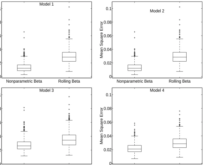
Figure 1 displays boxplots of the empirical distribution of MSE for each model and both esti-mators. More specifically, boxplots show graphically the median MSE, as well as the first quartile (q1) and third quartile (q3), the limits q3 +w(q3–q1) and q1–w(q3–q1) with w = 1.5, and values outside those limits. The figure shows that the first quartile, the median MSE and the third
quar-5
We orthogonalize the size factor by regressing Rsmb onRm. We then define the orthogonalized size factor as
the residuals from that regression. Next, we regressRhmlonRm and the orthogonalized size factor, and define the
tile are all lower for the nonparametric estimator than for the rolling estimator. The most striking difference is achieved for Model 1: The third quartile of the empirical MSE distribution is lower for the nonparametric estimator than the first quartile for the rolling estimator. We may therefore conclude that under the specifications considered, the nonparametric estimator clearly outperforms the rolling estimator in terms of providing more accurate estimates of betas.
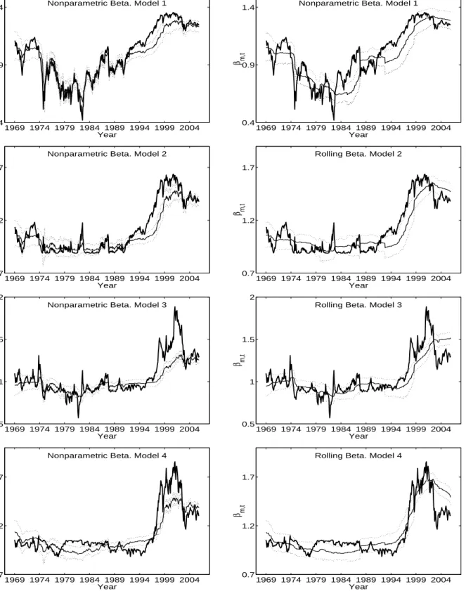
To gain further insight on the performance of the nonparametric estimator relative to the rolling estimator, in Figure 2 we plot the median, the first and the third quartiles of estimated betas for both estimators under the four specifications together with the true betas. The figure shows that the nonparametric estimator performs remarkably well under the four specifications, especially in the pre-1990 period. The median estimated beta tracks closely the true beta and the interquartile range is very narrow. The rolling estimator, in contrast, appears to respond slower to changes in the true beta. Also the interquartile range is substantially wider in all cases than for the nonparametric estimator.
6. Empirical application
In this section we apply the non-parametric method presented above to estimate conditional covariances and MPR in a flexible conditional version of the Fama and French (1993) three-factor model. By providing consistent estimates of time-varying market prices of risk as well as confidence intervals, our method makes it possible to identify time variation in the price of common risk factors. This is a desirable advantage over parametric methods that assume constant MPR since a statistically insignificant constant MPR associated with a risk factor may hide the fact that the risk factor is actually priced for certain subperiods or that the sign of the price has changed throughout the full sample period. We then compare the performance of the nonparametric approach to that of several alternatives that have been proposed in the literature in terms of their ability to predict the cross-section of future returns. This comparison enables us to establish whether the nonparametric approach leads to better estimates not only of factor sensitivities but also of MPR and, ultimately, asset expected returns.
6.1. Model and Data
We consider a particular case of the asset pricing relation (6) where the marketwide factors are the orthogonalized three Fama-French factors described in the previous section:
Like other studies, we use data on the 25 equity portfolios formed by sorting individual stocks on market capitalization and book-to-market (Fama and French (1993). Monthly data on the 25 portfolio returns and the one-month risk-free rate were downloaded from Kenneth French’s website. We follow closely Ferson and Harvey (1999) and select five conditioning variables (Xt−1) that
have been used in the literature on stock return predictability: (1) the annual dividend yield of the S&P 500 index (“DP”); (2) the slope of the term structure (“term”) as proxied by the difference between the yield on the ten-year Treasury bond and the yield on a one-year Treasury bill; (3) the default spread (“def”); (4) the one-month Treasury bill yield (“T b1m”); and (5) the difference between the monthly returns of a three-month and a one-month Treasury bill (“hb3”). DP,T b1m, and hb3 were constructed from data obtained from CRSP. Data on term and def were obtained from the Federal Reserve’s FRED database.
Our final sample contains 510 monthly observations of factor realizations, portfolio returns and lagged state variables in the July 1963-December 2005 period.
6.2. Estimation results
We start by estimating nonparametrically the conditional covariances of returns with the three risk factors and for each one of the 25 portfolios. We then estimate the time-varying market prices of risk associated with each factor.
To estimate conditional covariances at time t, we use 60 months of prior data on portfolio returns, factor realizations and conditioning variables. This results in a loss of 60 observations in the estimation of MPR. To mitigate the effects of the well-known curse of dimensionality that affects non-parametric estimation, we use only two conditioning variables at a time. More specifically, since DP has the most predictive power over future returns in univariate predictive regressions (unreported), we consider four pairs of conditioning variables, each one combiningDP with one of the remaining four state variables.
In Table 2 we report summary statistics of nonparametrically estimated MPR associated with the three Fama-French factors. For the sake of brevity, we report results only when the two conditioning variables are DP and term. Results for other choices of conditioning variables are similar and available from the authors upon request. Each panel in Table 2 shows the minimum, the mean, the standard deviation, and maximum values of ˆλm, ˆλsmb, and ˆλhml in a different subperiod. We also report the fraction of months in each subperiod in which estimated MPR are positive, and both positive and statistically significant at the 5% level. Results reveal that the prices associated with exposure to the market and the book-to-market risk factors are positive most of the time and with similar frequency: 84% and 84.67% of all months, respectively. However, the price of
book-to-market risk is statistically significant more often (about 29% of the time in the full sample) than the price of market risk (only 6% of all observations). The prices of risk associated with both risk factors are statistically significant more often in the 1996-2005 subperiod (15.83% and 35.83%, respectively) than in other subperiods. In contrast with these results, the price of the risk factor associated with size is negative on average in all subperiods with the exception of the 1976-1985 subperiod, and is positive only for 38.22% of all observations. Moreover, the price of size risk is never both positive and statistically significant. This price exhibits the highest standard deviation in the full sample. Interestingly, these results are broadly consistent with the finding by Ferson and Harvey (1999) that only the price of book-to-market risk is statistically significant in the 1963-1994 sample period.
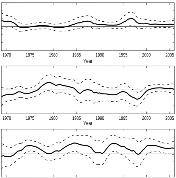
Figure 3 displays estimated MPR associated with the three Fama-French factors as well as 95% confidence intervals. Again, we report results obtained whenDP andtermare the only conditioning variables. The figure reveals that market prices of risk have varied substantially through time. Although the price of market risk has been consistently positive, it is not statistically significant most of the time, an important exception being the late nineties, when ˆλm reached its maximum value. Another interesting insight revealed by Figure 3 is that the price of size risk appears to have risen in the post-1999 period. Finally, although the book-to-market risk factor has been consistently priced by investors, the price associated with this risk factor appears to have varied through time: It achieved a peak in the early nineties and stayed at high levels again in the 2001-2005 period.
Taken together, our estimation results indicate that lack of significance of prices of the Fama-French market and size risk factors found by Ferson and Harvey (1999) survives a flexible speci-fication of the conditional FF model: Only the price of book-to-market risk is often positive and statistically significant. However, our results also suggest that MPR exhibit substantial variation through time. More specifically, the risk factor identified with the return on the market portfolio has been positive and significant in certain subperiods, even though the average price of this factor does not appear to be distinguishably different from zero.
6.3. Forecasting results
Ferson and Harvey (1999) test whether constant or linear FF factor betas can explain the cross-section of conditional expected returns against the alternative that conditional expected returns are captured by forecasts based on predictive OLS regressions of returns on lagged state variables. They find that including the OLS-forecast in cross-sectional regressions reduces the significance of Fama-MacBeth coefficients on both SMB and HML betas. Moreover, the coefficient on the OLS-forecast variable remains highly significant. They interpret these results as evidence against both
the unconditional and conditional versions of the FF model.
To evaluate the ability of the nonparametric approach to capture the cross-section of conditional expected returns, we perform a test that is similar to that employed by Ferson and Harvey (1999). First, for each month t we use information up to t−1 to estimate nonparametrically conditional covariances between asset returns and the risk factors. We also estimate the MPR corresponding to the last observation, i.e., bλt−1, and use them together with conditional covariances to compute
conditional expected returns, which we denote by ˆEN Pt−1(Rit). Like Ferson and Harvey (1999), for
each montht and each portfolioiin our sample, we also run the predictive OLS regression:
Ris=δ′it−1Xs−1+uis s= 1,2, ..., t−1, (37) and compute the fitted conditional expected return from the empirical model, ˆEtOLS−1 (Rit)≡ˆδ′it−1Xt−1.
We then estimate a series of cross-sectional regressions at each point in time:
Rit=φ0t+φN P tEˆtN P−1(Rit) +φOLStEˆtOLS−1 (Rit) +ηit i= 1,2, ..., N. (38)
Finally, the Fama-MacBeth coefficients are computed from the time series of regression coeffi-cients.6 The idea of the test is that under the null hypothesis that the conditional FF holds, we
would expect the estimated coefficient on ˆEN Pt−1(Rit) to be close to unity provided that our non-parametric approach yields accurate estimates of both conditional covariances and market prices of risk. Like Ferson and Harvey (1999), we include ˆEtOLS−1 (Rit) in the regression to confront the model
with a powerful empirically motivated alternative.
To put the results for the nonparametric model in perspective, we also estimate conditional expected returns from the parametric model. More specifically, we estimate the four parametric versions of the FF model considered by Ferson and Harvey (1999): (1) an unconditional FF model with betas estimated using expanding samples;7
(2) an unconditional FF model with betas esti-mated using 60-month rolling samples; (3) a conditional FF model with betas that are linear in the lagged state variables estimated using expanding samples;8
and (4) a conditional FF model with linear betas estimated using 60-month rolling samples. In all cases, rewards per unit of beta risk are estimated as the Fama-MacBeth coefficients from cross-sectional regressions of returns on betas
6
Regression (38) is run 330 months, which means that 180 observations are lost: 60 months of prior data are used to estimate conditional covariances; a minimum of 60 months of prior data are then used to estimate market prices of risk; and the first 60 return forecasts are used to choose the bandwidths that minimize forecasting errors.
7
The expanding sample used to estimate factor betas at timetincludes all observations from the first month to montht−1.
8
Linear betas are estimated from the time series regression: Rit = a0i + (bm0i+b′m1iXt−1)Rm,t +
over the previous 60 months.9 We use the notation ˆEP
t−1(Rit) to denote return forecasts implied
by the parametric implementation of the FF model.
Tables 3 and 4 report results for the nonparametric and the parametric estimation methods, respectively. To complete the analysis, we also report results from univariate regressions. The regression coefficient on the forecast based on the nonparametric FF model is positive, with values ranging from 0.67 to 0.91, and statistically significant at least at the 5% significance level in all cases. Moreover, none of of the intercepts is statistically significant. We interpret these results as evidence in favor of the flexible version of the conditional three-factor model. When the OLS-based forecast is included in the regression, the coefficient on ˆEtN P−1(Rit) is still positive in all cases but its
value decreases by half and becomes statistically insignificant. The coefficient on the OLS-based forecast, however, is statistically significant, although both its value and its statistical significance are lower than in the case in which ˆEOLS
t−1 (Rit) is the only regressor.
When returns are regressed on forecasts obtained from different parametric implementations of the FF model (Table 4), estimated slope coefficients are positive in all cases but lower than the coefficients obtained from the univariate regressions of Table 3, and they are never statistically significant. Interestingly, the lowest coefficients are obtained when betas are estimated using rolling samples rather than expanding samples. Further, the conditional model in which betas are allowed to vary linearly with the conditioning variables estimated with rolling samples provides the poorest fit: The slope coefficient takes the lowest value and the intercept becomes significant at the 5% level. If model-based forecasts are confronted with the OLS-based forecast, the coefficient on ˆEtP−1(Rit)
becomes negative in all cases although not significant at any conventional significance level, while the coefficient on ˆEtOLS−1 (Rit) remains high and statistically significant at the 1% level in all cases.
We may conclude from these results that our nonparametric approach to estimating the condi-tional FF model improves substantially upon alternative parametric methods in terms of forecasting the cross-section of future returns. However, nonparametric FF-based forecasts are still dominated by forecasts obtained from simple OLS regressions of returns on lagged state variables.
7. Summary and conclusions
In this paper we show how to estimate consistently time-varying market prices of risk in a general conditional beta pricing model without imposing any parametric structure on factor sensitivities or market prices of risk. The method can be seen as a nonparametric analogue of the two-pass approach developed by Fama and MacBeth (1973) to estimate and test unconditional beta pricing
9
In unreported results we also compute prices of beta risk as the average of the previous 30 regression coefficients and obtain qualitatively similar results.
models.
Like previously proposed nonparametric estimation methods, the method presented in this paper is not subject to Ghysels’ critique (Ghysels (1998), that misspecification of time-varying conditional moments and market prices of risk may induce larger pricing errors than those obtained by unconditional beta pricing models. Unlike previous proposals, however, ours does not assume that risk factors can be identified with portfolio returns, so it can be applied to a more general family of models. Moreover, our method provides estimates of both factor sensitivities and market prices of risk, which can be used to estimate expected returns for the purposes of forecasting future returns or estimating the cost of capital.
To evaluate the performance of the method in empirical analysis, we first carry out a simula-tion study and then apply the method to data on equity returns. Both analyses are based on the Fama-French three factor model. Simulation results suggest that the nonparametric methodology provides more accurate estimates of conditional betas than the traditional rolling-sample approach when beta depends on observable state variables. Estimation results using data on the 25 size and book-to-market sorted portfolios are consistent with prior evidence on the significance of market prices associated with the Fama-French risk factors. However, our results also suggest that infer-ence based on constant market prices of risk may hide that fact that risk factors are significantly priced in specific subperiods. Finally, our nonparametric version of the Fama-French model does a much better job at forecasting the cross-section of future stock returns than previously proposed parametric implementations, although the performance of the Fama-French model declines when confronted with purely empirical forecasts.
Appendix
In order to prove Theorem 1 the following lemma are needed.
Lemma 1 Under Assumptions (A2) to (A5), and (A8), it holds that
T X s=1 Kh,tsCs∗′Cs∗ a.s. −→Gt, (T h) T X s=1 K2 h,tsCs∗′Cs∗ p −→cKGt. Proof of Lemma 1
To simplify notation we denote any generic scalar term of T Kh,tsCs∗′Cs∗ asZs=T Kh,tsc∗sc∗s. Zs is aα−mixing sequence of size 6/5 with the proper bounded moments, andE(Zs) = h1K tT h−sgs, that tends togt. Therefore, the first result follows from the Strong Law of Large Numbers in White (1984), Corollary 3.48, for dependent variables under mixing conditions. The second result can be
proven following similar steps.
Proof of Theorem 1
First we write the Mean Square Error
M SE(λbt) = trE[(bλt−λt)(λbt−λt)′]
= ||Bias(bλt)||22 +trV ar(λbt) =S 2
(bλt) +V(bλt).
Then, note that
b λt−λt = T X s=1 Kh,tsCs∗′Cs∗ !−1 T X s=1 Kh,tsCs∗′R∗s−λt = T X s=1 Kh,tsCs∗′Cs∗ !−1 T X s=1 Kh,tsCs∗′Cs∗(λs−λt) + T X s=1 Kh,tsCs∗′Cs∗ !−1 T X s=1 Kh,tsCs∗′εs
has a random denominator. We overcome this problem redefining the bias and variance terms using the weightW∗
t =G−
1
t
PT
technical reasons, we use different bandwidths forW∗
t and for bλt, say h∗ and h respectively, such that the following condition holds:
EkW∗ t −I k2
Ekbλt−λtk2
=o(1), (39)
asT goes to infinity. This condition establishes thatW∗
t goes to the identity at a faster rate than the mean square error goes to zero, and this implies that the rate of convergence for the mean square error must be suboptimal, which in this case means slower thanT−4/5
. Considering the term defined by Bias∗
Bias∗(bλt) = G−t1 T X s=1 Kh,tsE(Cs∗′Cs∗)(λs−λt) +G−t1 T X s=1 Kh,tsE(Cs∗′ε∗s) = G−1 t T X s=1 Kh,tsE(Cs∗′Cs∗)(λs−λt),
sinceE(Cs∗′ε∗s) =E(Cs∗′E(ε∗s|Cs∗′)) = 0.Using the Taylor expansion with t−s=T hu,
Bias∗(bλt) = G−t1 T X s=1 Kh,tsGs(λs−λt) = G−t1 Z K(u) Gt−hu ∂Gt ∂t +o(h 2 ) −∂λt ∂t hu+ 1 2 ∂2 λt ∂t∂t(hu) 2 +o(h2 ) = 1 2dkh 2 ∂2λ t ∂t∂t + 2G −1 t ∂Gt ∂t ∂λt ∂t +o h2 . Thus, S2 (bλt) = 1 4d 2 kh 4 ∂2 λt ∂t∂t+ 2G −1 t ∂Gt ∂t ∂λt ∂t 2 2 +o(h4 ).
The variance term is given by
V ar(λbt) = V ar(bλt−λt) =V ar T X s=1 Kh,tsCs∗′Cs∗ !−1 T X s=1 Kh,tsCs∗′R∗s = V ar T X s=1 Kh,tsCs∗′Cs∗ !−1 T X s=1 Kh,tsCs∗′Cs∗(λs−λt) + T X s=1 Kh,tsCs∗′Cs∗ !−1 T X s=1 Kh,tsCs∗′εs ,
and using the redefined variance term, V ar∗(bλ t) =V ar(Wt∗bλt), it follows V ar∗(bλt) =V ar " G−1 t T X s=1 Kh,tsCs∗′Cs∗(λs−λt) # +V ar " G−1 t T X s=1 Kh,tsCs∗′εs # . (40)
Since the cross terms cancel because E(εs|Cs∗) = 0, the sum of variances can be split into two terms: V(bλt) = trV ar∗(bλt) =trV ar " G−1 t T X s=1 Kh,tsCs∗′Cs∗(λs−λt) # + trV ar " G−t1 T X s=1 Kh,tsCs∗′εs # =V1+V2. (41)
For the first term and taking into account that Gs=E(Cs∗′Cs∗) it follows
V1 = trV ar G−t1 T X s=1 Kh,tsCs∗′Cs∗(λs−λt) ! =trG−t1V ar T X s=1 Kh,tsCs∗′Cs∗(λs−λt) ! G−t1 = trG−1 t E T X s=1 Kh,ts Cs∗′Cs∗−Gs(λs−λt) T X s=1 Kh,ts Cs∗′Cs∗−Gs(λs−λt) !′ G−1 t = trG−t1E T X s=1 T X s′=1 Kh,tsKh,ts′ Cs∗′Cs∗−Gs(λs−λt)(λs′ −λt)′ Cs∗′′Cs∗′−Gs′ ! G−t1 = tr T X s=1 T X s′=1 Kh,tsKh,ts′(λs−λt)(λs′ −λt)′E Cs∗′′Cs∗′ −Gs′G−t1Gt−1 Cs∗′Cs∗−Gs = tr T X s=1 T X s′=1 Kh,tsKh,ts′(λs−λt)(λs′ −λt)′Qs,s′, (42) where Qs,s′ =E Cs∗′′C ∗ s′−Gs′
G−t1G−t1(Cs∗′Cs∗−Gs) is a bounded p-order square matrix. Ex-pression (42) can be divided in two parts, those corresponding to same terms and the cross terms. When s=s′ tr T X s=1 K2 h,ts(λs−λt)(λs−λt)′Qs,s,
whereQss is bounded and has same order as T X s=1 K2 h,ts(λs−λt)(λs−λt)′ = (T h)−1 Z K2 (u)(−hu∂λt ∂t +o(h))(−hu ∂λt ∂t +o(h)) ′du= = (T h−1)h2∂λt ∂t ∂λt ∂t ′Z u2K2(u)du +o(h2) =O h T .
For the cross terms, s6=s′
tr T X s,s′=1 s6=s′ Kh,tsKh,ts′(λs−λt)(λs′−λt)′Qs,s′
has same order as T X s,s′=1 s6=s′ Kh,tsKh,ts′(λs−λt)(λs′−λt)′=O h T + 1 T2 . ThusV1 =O Th + T12 .
For the second term in (41) and taking into account that E(ε∗
s|Cs∗) = 0: V2 = trV ar " G−t1 T X s=1 Kh,tsCs∗′ε∗s # =trG−t1V ar " T X s=1 Kh,tsCs∗′ε∗s # G−t1 = trG−t1E T X s=1 Kh,tsCs∗′ε∗s T X s=1 Kh,tsCs∗′ε∗s !′ G−t1 = trG−1 t E " T X s=1 T X s′=1 Kh,tsKh,ts′Cs∗′ε∗sε∗s′Cs∗′ # G−1 t .
Now, since E(εisεjs′) = 0 for all s6=s′,E(ε∗isε∗js′) = 0 and
V2 = trV ar " G−t1 T X s=1 Kh,tsCs∗′ε∗s # =trG−t1E " T X s=1 Kh,ts2 Cs∗′ε∗sε∗sCs∗ # G−t1 = trG−t1E " T X s=1 K2 h,tsCs∗′E(ε∗sε∗s|Cs∗)Cs∗ # G−t1.
Then, asE(ε∗
sε∗s|Cs∗) =I and using the result (39) of Lemma 1 we have that
V2 =trV ar " G−1 t T X s=1 Kh,tsCs∗′ε∗s # = ck T h trG −1 t GtG−t1+o((T h)− 1 ) = ck T h trG −1 t +o((T h)− 1 ).
Finally, since the order of V1 is negligible with respect toV2 and (39) holds, we have
V(bλ) = ck T h trG −1 t +o((T h)− 1 ),
from where it follows that the order of the leading term in the variance coincides with the order of
the variance term in standard results.
Proof of Corollary 1
Either condition (i) or (ii) provides, together with the rest of assumptions, the sufficient condi-tions of regularity to check that the convergence of Ωbs to Ωs implies the equivalence between the asymptotic properties of bλF GLS
t and bλt.
Proof of Proposition 1
In order to deal with the random denominator, we define the modified bias
Bias⋆(bciℓ(Xt−1)|Xt−1=xt−1) =Bias " 1 rf(τ, x′ t−1) t−1 X s=t−r KB(Xs−1−xt−1)bciℓ(xt−1) # withτ =t/T. Then Bias⋆(bciℓ(Xt−1)|Xt−1 =xt−1) = 1 rf(τ, x′ t−1) t−1 X s=t−r E[KB(Xs−1−xt−1)Piℓs]−f(τ, x′t−1)ciℓ(xt−1)
and, sincePiℓs =ciℓ(Xs−1) +us withE(us|Xs−1) = 0:
Bias⋆(bciℓ(Xt−1)|Xt−1 =xt−1) = 1 rf(τ, x′ t−1) t−1 X s=t−r E[KB(Xs−1−xt−1)ciℓ(Xs−1)]−f(τ, x′t−1)ciℓ(xt−1) = 1 rf(τ, x′ t−1) t−1 X s=t−r Z KB(ω−xt−1)ciℓ(ω)f s/T, ω′dω−f(t/T, x′t−1)ciℓ(xt−1) .
Now, define fs(x)≡f(s/T, x), Dc(xt−1)≡ ∂ciℓ(xt−1) ∂x1t−1 . . .∂ciℓ(xt−1) ∂xpt−1 ′ , Dfs(x ′ t−1)≡ ∂f s(x′t−1) ∂x1t−1 . . .∂fs(x ′ t−1) ∂xpt−1 ,
and the (p×p)-order matrices Hc(xt−1) andHfs(x′t−1) having as generic terms, (j, j′), ∂2c iℓ(xt−1) ∂xjt∂xj′t and ∂ 2 ∂fs(x′t−1) ∂xjt∂xj′t respectively.
Using a standard multivariate kernel of order two and the Lipschitz condition for the density
f; we have that Bias⋆(bciℓ(Xt−1)|Xt−1 =xt−1) = = 1 rf(τ, x′ t−1) t−1 X s=t−r Z K(z)ciℓ(xt−1+B1/2z)fs x′t−1+B 1/2 z′dz−ft(x′t−1)ciℓ(xt−1) = 1 rf(τ, x′ t−1) t−1 X s=t−r Z K(z) ciℓ(xt−1) + (B 1/2 z)′Dc(xt−1) + 1 2(B 1/2 z)′Hc(xt−1)(B 1/2 z) +o(trace(B)) × fs(x′t−1) + (B 1/2 z′)′Dfs(x ′ t−1) + 1 2(B 1/2 z′)′Hfs(x ′ t−1)(B 1/2 z′) +o(trace(B)) dz−ft(x′t−1)ciℓ(xt−1) = 1 rf(τ, x′ t−1) t−1 X s=t−r 1 2tr BHc(xt−1) Z K(z)zz′dz fs(x′t−1) + 1 rf(τ, x′ t−1) t−1 X s=t−r ciℓ(xt−1) fs(xt′−1)−ft(x′t−1) +O(trace(B)) = 1 rf(τ, x′ t−1) µK 2 tr(BHc(xt−1)) t−1 X s=t−r fs(x′t−1) + 1 rf(τ, x′ t−1) t−1 X s=t−r ciℓ(xt−1) fs(xt′−1)−ft(x′t−1) +O(trace(B)) = µK 2 tr(BHc(xt−1)) + 1 rf(τ, x′ t−1) t−1 X s=t−r ciℓ(xt−1)O r T +O(trace(B)) =O(trace(B)) +Or T .
V ar⋆(bciℓ(Xt−1)|Xt−1=xt−1) = 1 r2f2(τ, x′ t−1) V ar " t−1 X s=t−r KB(Xs−1−xt−1)piℓs # = 1 r2f2(τ, x′ t−1) " t−1 X s=t−r V ar(KB(Xs−1−xt−1)piℓs|xt−1) + t−1 X s,s′=t−r s6=s′
Cov(KB(Xs−1−xt−1)piℓs, KB(Xs′ −xt−1)piℓs′|xt−1) = 1 r2f2(τ, x′ t−1) " t−1 X s=t−r V ar(KB(Xs−1−xt−1)(ciℓ(xs−1) +uiℓs)|xt−1) + t−1 X s,s′=t−r s6=s′
Cov(KB(Xs−1−xt−1)(ciℓ(xs−1) +uiℓs), KB(Xs′−xt−1)(ciℓ(xs′) +uiℓs′)|xt−1) = 1 r2f2(τ, x′ t−1) " t−1 X s=t−r V ar(KB(Xs−1−xt−1) uiℓs|xt−1) + t−1 X s=t−r V ar(KB(Xs−1−xt−1)ciℓ(xs−1)|xt−1) + t−1 X s,s′=t−r s6=s′
Cov(KB(Xs−1−xt−1)ciℓ(Xs−1), KB(Xs′−1−xt−1)ciℓ(Xs′−1)|xt−1)
+ t−1 X
s,s′=t−r
s6=s′
Cov(KB(Xs−1−xt−1) uiℓs, KB(Xs′ −xt−1) uiℓs′|xt−1) = 1 r2f2(τ, x′ t−1) " t−1 X s=t−r V ar(KB(Xs−1−xt−1) uiℓs|xt−1) + t−1 X s=t−r V ar(KB(Xs−1−xt−1) ciℓ(xs−1)|xt−1) + t−1 X s,s′=t−r s6=s′
Cov(KB(Xs−1−xt−1)ciℓ(Xs−1), KB(Xs′−1−xt−1)ciℓ(Xs′−1)|xt−1)
=T1+T2+T3,
since fors6=s′the conditional expectationE(u
terms remain. For T1 T1 = 1 r2f2(τ, x′ t−1) " t−1 X s=t−r E(K2 B(Xs−1−xt−1)E(u2iℓs|Xs−1)|xt−1) # = σ 2 uiℓ r2f2(τ, x′ t−1) " t−1 X s=t−r E(KB2(Xs−1−xt−1)|xt−1) # = σ 2 uiℓ r2f2(τ, x′ t−1) " t−1 X s=t−r Z KB2(z−xt−1)f s/T, z′ dz # = σ 2 uiℓ r2f2(τ, x′ t−1)|B|1/2 t−1 X s=t−r Z K2 (u)f(τ, x′t−1) +O(traceB 1/2 ) +Or T du = σ 2 uiℓ rf(τ, x′ t−1)|B|1/2 Z K2 (u)du+h.o.t. =O 1 r|B|1/2 +h.o.t. For T2 T2 = 1 r2f2(τ, x′ t−1) t−1 X s=t−r V ar(KB(Xs−1−xt−1) ciℓ(xs−1)|xt−1) = 1 r2f2(τ, x′ t−1) t−1 X s=t−r "Z KB2(w−xt−1)c2iℓ(w)fs(w′)dw− Z KB(w−xt−1)ciℓ(w)fs(w′)dw 2# = 1 r2f2(τ, x′ t−1) t−1 X s=t−r |B|−1/2 Z K2 (z)c2 iℓ(xt−1+B1/2z)fs(x′t−1+B 1/2 z′)dz − Z K(z)ciℓ(xt−1+B1/2z)fs(x′t−1+B 1/2 z′)dz 2# = 1 r2f2(τ, x′ t−1)|B| 1/2 t−1 X s=t−r c2iℓ(xt−1)fs(x′t−1) Z K2(u)du+O(traceB1/2) −|B|1/2ciℓ(xt−1)fs(x′t−1) +O(traceB 1/2 ) 2 = c 2 iℓ(xt−1) r2f2(τ, x′ t−1)|B| 1/2 Z K2(u)du t−1 X s=t−r f(τ, x′t−1) +O(traceB 1/2 ) +Or T + h.o.t = c 2 iℓ(xt−1) rf(τ, x′ t−1)|B| 1/2 Z K2(u)du+h.o.t. = O 1 r|B|1/2 +h.o.t.
And finally for the third term, T3,
T3 = 1 r2f2(τ, x′ t−1) t−1 X s,s′=t−r s6=s′
Using (A4) r
X
k=1
Cov[KB(Xs−1−xt−1)ciℓ(Xs−1), KB(Xs+k−xt−1)ciℓ(Xs+k)|xt−1]
is uniformly bounded and, hence, the order ofT3 isO(r−1
), negligible with respect toT1 and T2. Therefore, the final expression for each (i, ℓ) variance term is
V ar⋆(bciℓ(Xt−1)|Xt−1 =xt−1) = c2 iℓ(xt−1) +σ2uiℓ rf(τ, x′ t−1)|B|1/2 Z K2 (u)du+h.o.t.
and the proof is complete.
Proof of Theorem 2
It is sufficient to check that the proof of Theorem 1 follows for the estimated covariances instead of the real ones. First, note that (A4) holds for the estimated covariances (Cb) and that (A5) holds up to ordero(1); that is, E(Cb∗′
t Cbt∗) =E(Ct∗′Ct∗) +o(1) =Gt+o(1).
Now, the steps of the proof of Theorem 1 follow straightforward using Cb instead of C. Only the second term for the variance (41) need an extra step.
The second term for the variance can be written as,
V ar G−t1 T X s=1 Kh,tsCbs∗′ε∗s ! = = G−1 t E E X s K2 h,tsCbs∗′ε∗sε∗′sCbs∗+ X s6=s′ Kh,tsKh,ts′Cbs∗′ε∗sε∗′s′Cbs∗′|Cbs∗ G−1 t = G−1 t E " X s K2 h,tsCbs∗′ε∗sε∗′sCbs∗+ X s<s′ Kh,tsKh,ts′Cbs∗′ε∗sE(ε∗′s′|Cbs∗,Cbs∗′, εs)Cbs∗′ +X s>s′ Kh,tsKh,ts′Cs∗′E(ε∗s|Cbs∗,Cbs∗′, εs′)ε∗′s′Cb ∗′ s′ # G−1 t = G−t1E " X s Kh,ts2 Cbs∗′ε∗sε∗′s′Cb ∗ s # G−t1,