Small Model for Economy of Iraq Based on
Semi-simulated Data
Salah H. Abid
Mathematics Department, Education College, Mustansiriyah University, Iraq
Abstract
In this paper, vector autoregressive model (VAR) is used to represent the most important variables in the Iraqi economy which are, Foreign Investment (FI), Iraqi Investment (II), Imports (IM), Exports (EX), Expenses (EXP), Income (IN), Broad Money (M2), Oil price (OI), Gross Domestic Product In Constant Price (2007=100) (GDP), Gross Foreign Assets of CBI (GF) and Exchange Rate in market price (ER). VAR model is estimated and some related tests are conducted. As a result, small model for economy of Iraq is obtained. To complete the work, principal component analysis is used for policy-making and prioritization for economy of Iraq. Most of information, approximately 86.13, is contained in three factors only. Based on the obtained results, all plans, policies and programs of economic and development in Iraq must be made according to the effects of factors and consequently variables under consideration.Keywords
Vector autoregressive model (VAR), Principal component analysis, Stability, Wald Test, Semi-simulated data, Akaike information criterion (AIC), Schwarz information criterion (SC)1. Introduction and Work Aims
The VAR model was introduced by Sims (1980) as a method to analyze macroeconomic data. He developed the VAR model as an alternative to the traditional system, which involved several equations.
Athanasopoulos et al in 2010 studied the joint determination of the lag length, the dimension of the cointegrating space and the rank of the matrix of short-run parameters of a vector autoregressive (VAR) model using model selection criteria. They considered model selection criteria which have data-dependent penalties as well as the traditional ones. They suggested a new two-step model selection procedure which is a hybrid of traditional criteria and criteria with data-dependant penalties and they proved its onsistency. Their Monte Carlo simulations measure the improvements in forecasting accuracy that can arise from the joint determination of lag-length and rank using their proposed procedure, relative to an unrestricted VAR or a cointegrated VAR estimated by the commonly used procedure of selecting the lag-length only and then testing for cointegration. Two empirical applications forecasting Brazilian inflation and U.S. macroeconomic aggregates growth rates respectively show the usefulness of the
* Corresponding author:
[email protected] (Salah H. Abid)
Published online at http://journal.sapub.org/economics
Copyright © 2019 The Author(s). Published by Scientific & Academic Publishing This work is licensed under the Creative Commons Attribution International License (CC BY). http://creativecommons.org/licenses/by/4.0/
model-selection strategy proposed here. The gains in different measures of forecasting accuracy are substantial, especially for short horizons.
Emmanuel in 2015 used the VAR models to model the Growth Domestics Products (GDP) of Ghana with other two selected macroeconomic such as inflation and real exchange rate for the period of 1980 to 2013. The empirical results derived, indicated that all the variables were stationary after their first differencing. The study further established that there is cointegration between macroeconomic variables and GDP in Ghana indicating long run relationship. The VECM (3) model was appropriately identified using AIC information criteria with co-integration relation of exactly one.
Kononenko in 2015 used VAR Methodology as well as Vector Error Correction (VEC) methodology to examine the existence and direction of causality between economic growth and IMF lending for Ukraine. The paper examines the IMF lending data for the period of 1991-2010. Robust empirical analysis indicates that IMF lending has a negative effect of on Ukraine's economic growth in the short term. Policy implications of this finding are that, despite short-run decline in economic growth, IMF lending can result in a long-run sustainable growth for Ukraine. For this, policymakers need to ensure that fund's money are used not only to cover budget's deficit, but also to finance institutional reforms.
across continuous and discrete time domain. They further clarified that the DVAR model of a continuous time, multivariate, linear Markov system is canonical under a highly generic condition. Their analysis shows that they can uniquely reproduced its SVAR and CTVAR models from the DVAR model. Based on these results, they proposed a novel Continuous and Structural Vector Autoregressive (CSVAR) modeling approach to derive the SVAR and the CTVAR models from their DVAR model empirically derived from the observed time series of continuous time linear Markov systems. They demonstrated its superior performance through some numerical experiments on both artificial and real-world data.
Gudeta et al in 2017 investigated the effect of export and import on real economic growth of Ethiopia. Yearly data set on the variables are obtained for the period 1982 to 2015 from national bank of the country. VAR analysis suggests that the lagged variables of both export and import have significant contributions in predicting the economic growth of the country.
In 2018, Forni et al resumed the line of research pioneered by Sims and Zha (Macroeconomic Dynamics, 2006, 10, 231–272) and make two novel contributions. First, they provided a formal treatment of partial fundamentalness, that is, the idea that a structural vector autoregression (VAR) can recover, either exactly or with good approximation, a single shock or a subset of shocks, even when the underlying model is nonfundamental. In particular, they extended the measure of partial fundamentalness proposed by Sims and Zha to the finite‐order case and study the implications of partial fundamentalness for impulse‐response and variance‐decomposition analysis. Second, they presented an application where they validated a theory of news shocks and found it to be in line with the empirical evidence.
Huber and Pfarrhofer in 2019 provided a parsimonious means to estimate panel VARs with stochastic volatility. They assumed that coefficients associated with domestic lagged endogenous variables arise from a Gaussian mixture model. Shrinkage on the cluster size was introduced through suitable priors on the component weights and cluster-relevant quantities were identified through novel shrinkage priors. To assess whether dynamic interdependencies between economies are needed, they moreover impose shrinkage priors on the coefficients related to other countries’ endogenous variables. Finally, their model controls for static interdependencies by assuming that the reduced form shocks of the model feature a factor stochastic volatility structure. They assessed the merits of the proposed approach by using synthetic data as well as a real data application. In the empirical application, they forecast Eurozone unemployment rates and shows that their proposed approach works well in terms of predictions.
Hecq et al in 2019 developed an LM test for Granger causality in high-dimensional VAR models based on penalized least squares estimations. To obtain a test which retains the appropriate size after the variable selection done by the lasso, they proposed a post-double selection
procedure to partial out the effects of the variables not of interest. They conducted an extensive set of Monte-Carlo simulations to compare different ways to set up the test procedure and choose the tuning parameter. The test performs well under different data generating processes, even when the underlying model is not very sparse. They investigated also two empirical applications: the money-income causality relation using a large macroeconomic dataset and networks of realized volatilities of a set of 49 stocks. In both applications they find evidences that the causal relationship becomes much clearer if a high- dimensional VAR is considered compared to a standard low-dimensional one.
Aikman in 2019 presented a methodology for modelling the interaction between quantiles of endogenous variables in a VAR. They apply this to a bivariate quantile VAR on euro area data for industrial production and a financial stress indicator. They find that financial shocks shift the shape of the distribution of industrial production in the short term, increasing the fatness of the tail.
Owing to its simplicity and less restrictions, the vector autoregressive with exogenous variable (VARX) model is one of the statistical analyses frequently used in many studies involving time series data, such as finance, economics, and business. PTBA and HRUM energy as endogenous variables and exchange rate as an exogenous variable were studied by Warsono in 2019. The data used were collected from January 2014 to October 2017. The dynamic behavior of the data was also studied through IRF and Granger causality analyses. The forecasting data for the next 1 month was also investigated. On the basis of the data provided by these different models, it was found that VARX (3,0) is the best model to assess the relationship between the variables considered in this work.
In this paper, we have two aims, the first one is the modeling of most important variables of Iraqi economy, model estimation and related issues. The second aim is the policy-making and prioritization for economy of Iraq.
2. VAR Process Model
The vector autoregression (VAR) is usually used for forecasting systems of interconnected time series and for analyzing the influence of random errors on the system of variables. VAR processes are common in economics because they are easy and ductile models for multivariate time series data. Var models became standard tools since Sims (1980) contested the way traditional simultaneous equations models were named, recognized and recommended these models as alternatives. These models are treated in depth in books of Lütkepohl (2005) and Hamilton (1994). VAR models does not need for structural modeling by considering every endogenous variable as a function of the lagged values of all of the endogenous variables in the system. Suppose that we interested in a set of 𝑚 related time series variables collected in 𝑦𝑡 = 𝑦1𝑡, 𝑦2𝑡, … , 𝑦𝑚𝑡 𝑇.
𝑦𝑡 = 𝐵𝑏𝑡+ 𝐴1𝑦𝑡−1+ 𝐴2𝑦𝑡−2+ ⋯ + 𝐴𝑝𝑦𝑡−𝑝+ 𝑢𝑡 (1)
Where 𝑦𝑡 is a 𝑚 vector of endogenous variables, 𝐴𝑖 (𝑖 = 1,2, … , 𝑝) are (𝑚 × 𝑚) matrices of parameters, 𝑏𝑡is a vector of deterministic terms such as a constant, a
linear trend and/or seasonal, 𝐵 is the matrix of parameters related with 𝑏𝑡, and 𝑢𝑡 is a vector of errors that may be
jointly correlated but are uncorrelated with their own lagged values and uncorrelated with all of the right-hand side variables. The error process 𝑢𝑡 is assumed to be white noise
with zero mean, that is, (𝑢𝑡) = 0, the covariance matrix, 𝐸 𝑢𝑡𝑢𝑡𝑇 = 𝛴𝑢 , is time invariant and the 𝑢𝑡’s are serially
uncorrelated or independent.
By using the lag operator 𝐴(𝐿) = 𝐼𝑚− 𝐴1𝐿 − ⋯ − 𝐴𝑝𝐿𝑝, (1) can be reformed as,
𝐴(𝐿) 𝑦𝑡− 𝐵𝑏𝑡 = 𝑢𝑡 (2)
The VAR process is stable if all roots of the determinantal polynomial are outside the complex unit circle, which is mean that, 𝐷𝑒𝑡 𝐴(𝜔) ≠ 0 for 𝜔 ∈, 𝜔 ≤ 1. Since that any stable process 𝑦𝑡 has time invariant means, variances and
covariance structure and is, hence, stationary.
VAR models are suited tools for forecasting. If the 𝑢𝑡’s
are independent white noise, the minimum mean squared error (MSE) h-step forecast of 𝑦𝑡+ℎ at time t is the
conditional expectation given 𝑦𝑠, 𝑠 ≤ 𝑡, 𝑦 𝑡+ℎ 𝑡= 𝐸 𝑦𝑡+ℎ 𝑦𝑡, 𝑦𝑡−1, …
=𝐵𝑏𝑡+ℎ+ 𝐴1𝑦 𝑡+ℎ−1 𝑡+ 𝐴2𝑦 𝑡+ℎ−2 𝑡+ ⋯ + 𝐴𝑝𝑦 𝑡+ℎ−𝑝 𝑡 (3)
Where 𝑦 𝑡+𝑖 𝑡=𝑦𝑡+𝑖 for 𝑖 ≤ 0. Using this formula, the
forecasts can be computed recursively for ℎ = 1,2, …. The forecasts are unbiased, that is, the forecast error 𝑦𝑡+ℎ− 𝑦 𝑡+ℎ 𝑡 has mean zero and the forecast error covariance is equal to the MSE matrix. The one-step ahead forecast errors are the 𝑢𝑡’s.
VAR models can also be consumed for analyzing the connections among variables involved. For example, Granger (1969) determined a notion of causality which given that a variable 𝑦1𝑡 is causal for a variable 𝑦2𝑡 if the
information in 𝑦1𝑡 is beneficial for ameliortating the
forecasts of 𝑦2𝑡. If the two variables are jointly generated by
a VAR process, it turns out that 𝑦1𝑡 is not Granger-causal
for 𝑦2𝑡 if a simple set of zero conditions for the VAR model
coefficients are fulfilled. Hence, Granger-causality is light to check in VAR processes.
2.1. Estimation and Model Specification
Usually, in practical applications, the process which has generated the time series under study is unknown. So, if VAR models are considered as appropriate, the lag order has to be determined and the parameters have to be estimated. Consequently, for a given VAR of order p, estimation can be well done by the ordinary least squares (OLS). For a sample of size 𝑘 , 𝑦1, 𝑦2, … , 𝑦𝑘, and assuming that moreover initial
values 𝑦−𝑝+1, … , 𝑦0 are available, the OLS estimator of the
parameters 𝑄 = 𝐵, 𝐴1, … , 𝐴𝑝 will be,
𝑄 = 𝑘𝑡=1𝑦𝑡𝑣𝑡−1𝑇 𝑘𝑡=1𝑣𝑡−1𝑣𝑡−1𝑇 −1 (4)
Where, 𝑣𝑡−1𝑇 = 𝑏𝑡𝑇, 𝑦𝑡−1𝑇 , … , 𝑦𝑡−𝑝𝑇 . Under standard
assumptions the estimator is consistent and asymptotically normally distributed. Actually, if the residuals and, hence, the 𝑦𝑡’s are normally distributed, that is, 𝑢𝑡~ 0, 𝛴𝑢 , the
OLS estimator is equal to the maximum likelihood (ML) estimator with the usual asymptotic optimality properties. It is well known that, the number of parameters is also large, when the dimension 𝑚 of the process is large, then the estimation precision may be low if a sample of typical size in macroeconomic studies is available for estimation. In that case, it may be opportune to use so-called subset VAR models by estranging excessive lags of some of the variables from some of the equations. Generally, other estimation methods may be more efficient if some restrictions are enjoined on the parameter matrices.
By the following most popular model selection criteria, VAR order selection is usually done,
1. Akaike’s information criterion (AIC) (Akaike, 1973), with the form,
𝐴𝐼𝐶(𝑙) = 𝐿𝑜𝑔 𝐷𝑒𝑡(𝛴 𝑙) + 2𝑙𝑚2 𝑘
2. Hannan-Quinn criterion (HQC) (Hannan and Quinn, 1979), with the form,
𝐻𝑄𝐶(𝑙) = 𝐿𝑜𝑔 𝐷𝑒𝑡(𝛴 𝑙) + 2𝑙𝑚2 𝐿𝑜𝑔 𝐿𝑜𝑔(𝑘) 𝑘
Where, 𝛴 𝑙 = 𝑘𝑡=1𝑢 𝑡𝑢 𝑡𝑇 is the residual covariance matrix
of a VAR(𝑙) model estimated by OLS. The VAR order is chosen which perfectly equipoises both terms. Factually, models of orders 𝑙 = 0,1, … , 𝑝𝑚𝑎𝑥 are estimated and the
order 𝑝 is chosen such that it minimizes the value of the criteria.
The fact that 𝐴𝐼𝐶 < 𝐻𝑄𝐶 implies to that the 𝐻𝑄𝐶 generally chooses models with a smaller 𝑝 while AIC chooses models with a higher order 𝑝.
Once a model is estimated it should be checked that it represents the data features sufficiently.
If some of the time series variables to be modeled with a VAR have stochastic trends, that is, they manage similarly to a random walk, and then another model framework may be more suitable for analyzing especially the trending properties of the variables. Stochastic trends in some of the variables are generated by models with unit roots in the VAR operator, that is 𝐷𝑒𝑡 𝐼𝑚− 𝐴1𝜔 − ⋯ − 𝐴𝑝𝜔𝑝 = 0, for 𝜔 = 1.
Variables with such trends are nonstationary and not stable. They are often called integrated. They can be made stationary by differencing. Furthermore, they are called cointegrated if stationary linear combinations exist or, in other words, if some variables are driven by the same stochastic trend. Cointegration relations are often of specific benefit in economic studies. In that case, reparameterizing the standard VAR model such that the cointegration relations appear immediately may be appropriate. The so-called vector error correction model (VECM) of the form,
∆𝑦𝑡 = 𝐵𝑏𝑡+ 𝛩𝑦𝑡−1+ 𝛷1∆𝑦𝑡−2+ ⋯ + 𝛷𝑝−1∆𝑦𝑡−𝑝+1+ 𝑢𝑡
(5) is a simple example of such a reparametrization, where
∆ denotes the differencing operator defined such that,
−𝐴𝑖+1− ⋯ − 𝐴𝑝 for (𝑖 = 1, … , 𝑝 − 1). This
parametrization is acquired by subtracting 𝑦𝑡−1 from both
sides of the standard VAR formulation and rearranging terms. Its merit is that 𝛩 can be decomposed such that the cointegration relations are straight sitting in the model. More accurately, if all variables are stationary after differencing once, and there are 𝑚 − 𝑟 common trends, then the matrix
𝛩 has rank 𝑟 and can be decomposed as, 𝛩 = 𝛿𝛾𝑇, where
𝛿 and 𝛾 are (𝑚 × 𝑟) matrices of rank 𝑟 and 𝛾 includes the cointegration relations. A detailed statistical analysis of this model is offered in Johansen (1995).
3. Model of Iraqi Economy
In this section, a small model for economy of Iraq will presented according to data obtained from the website of central bank of Iraq. The variables used here are Foreign Investment (FI), Iraqi Investment (II), Imports (IM), Exports (EX), Expenses (EXP), Income (IN), Broad Money (M2), Oil price (OI), Gross Domestic Product In Constant Price (2007=100) (GDP), Gross Foreign Assets of CBI (GF) and Exchange Rate in market price (ER). The data shown in table (1) in appendix. Three of variables IM, EX and GDP have been compiled on an annual basis, while the other variables were compiled on a monthly basis. To unify these basis, we estimated three annual models based on time as independent variables to simulate the monthly values of these variables. The models are as follows,
IM= 659.491 𝑡 - 2.36437 𝑡2 + 0.0271158 𝑡3
- 0.000175894 𝑡4 (6) With adjusted determination coefficient 𝑅4 equal to 97.9491 and mean square error equal to 4.1018E7.
Ex = 0.538477 𝑡 + 0.0105689 𝑡2 - 0.0000988688 𝑡3 + 1.55976E-7 𝑡4 (7)
With adjusted determination coefficient 𝑅4 equal to 93.9906 and mean square error equal to 248.287.
GDP = 6.53025 𝑡 - 0.121239 𝑡2 + 0.000946019 𝑡3
- 0.00000245094 𝑡4 (8) With adjusted determination coefficient 𝑅4 equal to 99.1058 and mean square error equal to 229.995.
Three models are accepted to represent data according to F-ANOVA test at all popular significant levels 0.01, 0.05 and 0.10. The simulated data are recognized by red color in table (1) and the variables which are simulated will recognized by letter s, to be GDPS instead of GDP, EXS instead of EX and IMS instead of IM.
We will present our work according to the following steps, (1) The VAR model is considered. Table (1) shows the results of model estimation. The estimates of model parameters are in the first line at each of independent variables. The second line contains the standard deviation for each corresponding estimate while the third line contains the computed t- statistic to test the null hypothesis, which is said that the parameter under consideration is equal to zero, against the alternative hypothesis, which is not said that. The p-value is contained in the fourth line. The bold font for the p-values is used to recognize the rejected hypotheses, which is meaning that the variable has an effect.
(2) The values of Adj. R-squared, Log likelihood, Akaike AIC and Schwarz SC in table (1), show that the model is worked well done.
(3) The initial VAR model (which is contained all considered independent variables and lagged variables of order 2 according to criteria in table (2)) is as follows,
𝐸𝑅 = 1.292 𝐸𝑅−1- 0.351 𝐸𝑅−2 - 0.00028 𝐺𝐹−1 - 0.0003388 𝐺𝐹−2 - 0.4237 𝑂𝐼−1 + 0.4995 𝑂𝐼−2 + 1.504 𝐺𝐷𝑃𝑆−1 -
2.91 𝐺𝐷𝑃𝑆−2 - 2.455e-07 𝐸𝑋𝑃−1 + 1.6565e-07 𝐸𝑋𝑃−2 + 1.4167e-07 𝐼𝑁−1 - 1.385e-07 𝐼𝑁−2 - 4.4675 𝐸𝑋𝑆−1+
1.333 𝐸𝑋𝑆−2 - 0.00356 𝐼𝑀𝑆−1+ 0.0051 𝐼𝑀𝑆−2 - 1.223e-05 𝐹𝐼−1+ 9.89e-06 𝐹𝐼−2- 3.327e-06 𝐼𝐼−1+ 1.6e-06 𝐼𝐼−2+
4.38e-07 𝑀2−1+ 2.5475e-07 𝑀2−2+ 100.55
𝐺𝐹 = - 3.36 𝐸𝑅−1 - 5.724 𝐸𝑅−2 + 0.61435 𝐺𝐹−1 + 0.2188 𝐺𝐹−2 - 10.226 𝑂𝐼−1 + 49.55 𝑂𝐼−2 - 308.625 𝐺𝐷𝑃𝑆−1
+ 282.808 𝐺𝐷𝑃𝑆−2 + 4.912e-05 𝐸𝑋𝑃−1 - 1.409e-05 𝐸𝑋𝑃−2 - 3.582e-05 𝐼𝑁−1 + 7.295e-06 𝐼𝑁−2 + 253.25 𝐸𝑋𝑆−1 +
43.7688 𝐸𝑋𝑆−2 + 0.37053 𝐼𝑀𝑆−1 - 0.267 𝐼𝑀𝑆−2 + 0.000244 𝐹𝐼−1- 0.000241 𝐹𝐼−2+ 3.0417e-05 𝐼𝐼−1 -
0.0002017 𝐼𝐼−2+ 2.89e-05 𝑀2−1+ 3.073e-05 𝑀2−2 + 12748.07
𝑂𝐼 = 0.03761*𝐸𝑅−1- 0.036 𝐸𝑅−2 + 6.4681e-05 𝐺𝐹−1 + 2.9723e-05 𝐺𝐹−2 + 1.489 𝑂𝐼−1 - 0.6038 𝑂𝐼−2 - 1.0554 𝐺𝐷𝑃𝑆−1 + 0.4211 𝐺𝐷𝑃𝑆−2 + 1.089e-07 𝐸𝑋𝑃−1 + 1.211e-08 𝐸𝑋𝑃−2 - 1.0204e-07 𝐼𝑁−1 - 3.272e-08 𝐼𝑁−2 + 1.665 𝐸𝑋𝑆−1 + 0.2634 𝐸𝑋𝑆−2 + 0.00053 𝐼𝑀𝑆−1- 0.001153 𝐼𝑀𝑆−2- 2.921e-07 𝐹𝐼−1 + 2.9576e-07 𝐹𝐼−2+ 1.293e-07 𝐼𝐼−1-
6.691e-08 𝐼𝐼−2- 1.2737e-07 𝑀2−1+ 8.339e-08 𝑀2−2+ 6.684
𝐺𝐷𝑃𝑆 = 0.0054753*𝐸𝑅−1- 0.00533 𝐸𝑅−2 - 1.270648e-05 𝐺𝐹−1 + 1.11512e-05 𝐺𝐹−2 + 0.01916 𝑂𝐼−1 - 0.02474 𝑂𝐼−2 + 0.84514 𝐺𝐷𝑃𝑆−1 - 0.1086 𝐺𝐷𝑃𝑆−2 - 1.372e-08 𝐸𝑋𝑃−1 + 7.363e-09 𝐸𝑋𝑃−2 + 1.4514e-08 𝐼𝑁−1 - 6.055e-09 𝐼𝑁−2 - 0.02621 𝐸𝑋𝑆−1 + 0.07958 𝐸𝑋𝑆−2 - 0.00026 𝐼𝑀𝑆−1- 4.0256e-05 𝐼𝑀𝑆−2- 1.93478e-07 𝐹𝐼−1+
1.55591e-07 𝐹𝐼−2- 5.02166e-08 𝐼𝐼−1 + 3.1218e-08 𝐼𝐼−2- 9.6437e-08 𝑀2−1+ 1.30627e-07 𝑀2−2+ 2.581
𝐸𝑋𝑃 = - 20063.186*𝐸𝑅−1+ 29132.994 𝐸𝑅−2 - 1469.215 𝐺𝐹−1 + 1579.646 𝐺𝐹−2 + 147402.404 𝑂𝐼−1 + 125033.64 𝑂𝐼−2 + 1092145.579 𝐺𝐷𝑃𝑆−1 - 21436.69 𝐺𝐷𝑃𝑆−2 + 0.1897 𝐸𝑋𝑃−1 + 0.13856 𝐸𝑋𝑃−2 + 0.40743 𝐼𝑁−1 - 0.235 𝐼𝑁−2 - 3191803.31 𝐸𝑋𝑆−1 - 341863.69 𝐸𝑋𝑆−2 + 2327.7 𝐼𝑀𝑆−1- 528.95 𝐼𝑀𝑆−2- 5.4258 𝐹𝐼−1+ 3.821 𝐹𝐼−2-
𝐼𝑁 = - 163957.477*𝐸𝑅−1+ 197231.444 𝐸𝑅−2 - 1755.3933 𝐺𝐹−1 + 2066.1762 𝐺𝐹−2 + 212580.87 𝑂𝐼−1 +
391844.534 𝑂𝐼−2 + 1753313.7254 𝐺𝐷𝑃𝑆−1 + 34403.7 𝐺𝐷𝑃𝑆−2 - 0.141078 𝐸𝑋𝑃−1 - 0.0610626 𝐸𝑋𝑃−2 + 0.7207 𝐼𝑁−1 - 0.13178 𝐼𝑁−2 - 5292199.22 𝐸𝑋𝑆−1 - 704813.2 𝐸𝑋𝑆−2+ 4248.33 𝐼𝑀𝑆−1- 1511.43 𝐼𝑀𝑆−2- 6.58571 𝐹𝐼−1+
4.6481 𝐹𝐼−2- 1.461 𝐼𝐼−1+ 2.5451 𝐼𝐼−2- 4.40613 𝑀2−1+ 4.2039 𝑀2−2- 68251824.82
𝐸𝑋𝑆 = 0.0007692*𝐸𝑅−1- 0.000873 𝐸𝑅−2 + 1.15629e-05 𝐺𝐹−1 - 1.8591e-05 𝐺𝐹−2 + 0.0197 𝑂𝐼−1 - 0.00092 𝑂𝐼−2
+ 0.00977 𝐺𝐷𝑃𝑆−1 - 0.01995 𝐺𝐷𝑃𝑆−2 - 1.45756e-09 𝐸𝑋𝑃−1 + 5.7589e-09 𝐸𝑋𝑃−2 + 1.1807e-10 𝐼𝑁−1 -
4.161232e-09 𝐼𝑁−2 + 0.6341 𝐸𝑋𝑆−1 + 0.0682 𝐸𝑋𝑆−2 + 8.020e-05 𝐼𝑀𝑆−1- 0.0001 𝐼𝑀𝑆−2- 3.58e-08 𝐹𝐼−1-
1.204e-09 𝐹𝐼−2- 9.8478e-08 𝐼𝐼−1+ 9.9565e-08 𝐼𝐼−2- 2.58e-08 𝑀2−1+ 3.9371e-08 𝑀2−2+ 0.14377
𝐼𝑀𝑆 = 2.1868*𝐸𝑅−1- 2.41268 𝐸𝑅−2 + 0.003263 𝐺𝐹−1 - 0.00312 𝐺𝐹−2 + 6.939 𝑂𝐼−1 - 4.6393 𝑂𝐼−2 - 26.4994 𝐺𝐷𝑃𝑆−1 - 12.9734 𝐺𝐷𝑃𝑆−2 - 2.685e-06 𝐸𝑋𝑃−1 + 2.57169e-06 𝐸𝑋𝑃−2 + 2.5098e-06 𝐼𝑁−1 - 1.773625e-06 𝐼𝑁−2 -
46.2467 𝐸𝑋𝑆−1 + 32.53676 𝐸𝑋𝑆−2+ 0.9272 𝐼𝑀𝑆−1- 0.0778 𝐼𝑀𝑆−2+ 4.545e-05 𝐹𝐼−1 - 6.499e-05 𝐹𝐼−2-
5.679e-06 𝐼𝐼−1- 2.3959e-06 𝐼𝐼−2- 1.73862e-05 𝑀2−1 + 2.4863e-05 𝑀2−2+ 847.86
𝐹𝐼 = 1946.34*𝐸𝑅−1+ 1281.74 𝐸𝑅−2 + 7.097 𝐺𝐹−1 + 30.406 𝐺𝐹−2 + 4517.77 𝑂𝐼−1 - 6680.866 𝑂𝐼−2 + 15972.33 𝐺𝐷𝑃𝑆−1 - 15893.8573 𝐺𝐷𝑃𝑆−2 + 0.0009 𝐸𝑋𝑃−1 + 0.00073 𝐸𝑋𝑃−2 - 0.000717 𝐼𝑁−1 - 0.00137 𝐼𝑁−2 + 26077.564 𝐸𝑋𝑆−1 - 39725.965 𝐸𝑋𝑆−2- 161.0082 𝐼𝑀𝑆−1+ 127.9697 𝐼𝑀𝑆−2+ 0.84961 𝐹𝐼−1- 0.05567 𝐹𝐼−2- 0.011626 𝐼𝐼−1+
0.11277 𝐼𝐼−2+ 0.0012364 𝑀2−1- 0.02178 𝑀2−2- 4394115.7
𝐼𝐼 = - 3543.093*𝐸𝑅−1+ 159.5519 𝐸𝑅−2 - 34.301 𝐺𝐹−1 + 0.3739 𝐺𝐹−2 - 12075.02 𝑂𝐼−1 + 19601.485 𝑂𝐼−2 +
24823.637 𝐺𝐷𝑃𝑆−1 + 27680.25 𝐺𝐷𝑃𝑆−2 - 0.006797 𝐸𝑋𝑃−1 - 0.002719 𝐸𝑋𝑃−2 + 0.00537 𝐼𝑁−1 - 0.00074 𝐼𝑁−2 -
152482.92 𝐸𝑋𝑆−1 - 50657.1691 𝐸𝑋𝑆−2 - 69.773 𝐼𝑀𝑆−1+ 91.788 𝐼𝑀𝑆−2+ 0.10014 𝐹𝐼−1- 0.082 𝐹𝐼−2 + 1.0953 𝐼𝐼−1-
0.242 𝐼𝐼−2 + 0.0329 𝑀2−1 - 0.00323 𝑀2−2+ 4727355.5
𝑀2 = 13659.4366*𝐸𝑅−1- 13933.864 𝐸𝑅−2 - 44.234 𝐺𝐹−1 + 89.1996 𝐺𝐹−2 - 11745.15 𝑂𝐼−1+ 28321.38 𝑂𝐼−2 +
249914.34 𝐺𝐷𝑃𝑆−1 - 99876.7868 𝐺𝐷𝑃𝑆−2 - 0.003586 𝐸𝑋𝑃−1 + 0.00965 𝐸𝑋𝑃−2 + 0.010561 𝐼𝑁−1 - 0.0156 𝐼𝑁−2 -
168245.3197 𝐸𝑋𝑆−1 - 52714.051 𝐸𝑋𝑆−2- 747.871542 𝐼𝑀𝑆−1+ 645.5 𝐼𝑀𝑆−2- 0.3181 𝐹𝐼−1- 0.12795 𝐹𝐼−2+
0.05816 𝐼𝐼−1+ 0.064677 𝐼𝐼−2+ 0.881 𝑀2−1+ 0.072087 𝑀2−2+ 98509.199
(9)
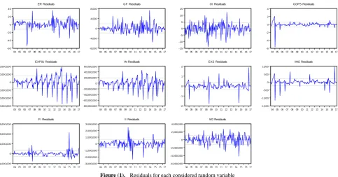
Graph (1) represent the residuals for each considered random variable,
-60 -40 -20 0 20 40
04 05 0607 08 0910 11 1213 14 1516 17
ER Residuals -8,000 -4,000 0 4,000 8,000
04 0506 0708 09 1011 12 1314 15 16 17
GF Residuals -15 -10 -5 0 5 10 15
04 05 0607 08 0910 11 1213 14 1516 17
OI Residuals -6 -4 -2 0 2 4
0405 06 0708 09 1011 12 1314 15 16 17
GDPS Residuals -60,000,000 -40,000,000 -20,000,000 0 20,000,000 40,000,000
04 05 0607 08 0910 11 1213 14 1516 17
EXP01 Residuals
-80,000,000 -60,000,000 -40,000,000 -20,000,000 0 20,000,000 40,000,000 60,000,000
04 0506 0708 09 1011 12 1314 15 16 17
IN Residuals -2 -1 0 1 2
04 05 0607 08 0910 11 1213 14 1516 17
EXS Residuals -1,500 -1,000 -500 0 500 1,000
0405 06 0708 09 1011 12 1314 15 16 17
IMS Residuals -1,000,000 0 1,000,000 2,000,000 3,000,000
04 05 0607 08 0910 11 1213 14 1516 17
FI Residuals -3,000,000 -2,000,000 -1,000,000 0 1,000,000 2,000,000 3,000,000
04 0506 0708 09 1011 12 1314 15 16 17
II Residuals -6,000,000 -4,000,000 -2,000,000 0 2,000,000 4,000,000
04 05 0607 08 0910 11 1213 14 1516 17
M2 Residuals
Figure (1). Residuals for each considered random variable
𝐸𝑅 = 100.55- 0.4237 𝑂𝐼−1 + 0.4995 𝑂𝐼−2 - 1.223e-05 𝐹𝐼−1+ 9.89e-06 𝐹𝐼−2- 3.327e-06 𝐼𝐼−1+4.38e-07 𝑀2−1+
2.5475e-07 𝑀2−2
𝐺𝐹 = 12748.07 + 0.61435 𝐺𝐹−1 + 0.2188 𝐺𝐹−2 + 4.912e-05 𝐸𝑋𝑃−1 - 3.582e-05 𝐼𝑁−1 - 3.36 𝐸𝑅−1 - 5.724 𝐸𝑅−2 -
10.226 𝑂𝐼−1 + 49.55 𝑂𝐼−2
𝑂𝐼 = 1.489 𝑂𝐼−1 - 0.6038 𝑂𝐼−2 + 1.089e-07 𝐸𝑋𝑃−1 - 1.0204e-07 𝐼𝑁−1 + 1.665 𝐸𝑋𝑆−1 + 0.2634 𝐸𝑋𝑆−2 𝐺𝐷𝑃𝑆 = 0.01916 𝑂𝐼−1 - 0.02474 𝑂𝐼−2 + 0.84514 𝐺𝐷𝑃𝑆−1 + 1.4514e-08 𝐼𝑁−1 - 9.6437e-08 𝑀2−1+
1.30627e-07 𝑀2−2
𝐸𝑋𝑃 = - 1469.215 𝐺𝐹−1 + 1579.646 𝐺𝐹−2 + 0.40743 𝐼𝑁−1 - 3.73872 𝑀2−1+ 3.68252* 𝑀2−2
𝐼𝑁 = 197231.444 𝐸𝑅−2 - 1755.3933 𝐺𝐹−1 + 2066.1762 𝐺𝐹−2 + 0.7207 𝐼𝑁−1 - 4.40613 𝑀2−1+ 4.2039 𝑀2−2+
212580.87 𝑂𝐼−1 + 391844.534 𝑂𝐼−2
𝐸𝑋𝑆 = 0.0197 𝑂𝐼−1 + 0.6341 𝐸𝑋𝑆−1 - 9.8478e-08 𝐼𝐼−1+ 9.9565e-08 𝐼𝐼−2- 2.58e-08 𝑀2−1+ 3.9371e-08 𝑀2−2 𝐼𝑀𝑆 = 2.1868*𝐸𝑅−1- 2.41268 𝐸𝑅−2 + 6.939 𝑂𝐼−1 + 0.9272 𝐼𝑀𝑆−1- 26.4994 𝐺𝐷𝑃𝑆−1 - 12.9734 𝐺𝐷𝑃𝑆−2-
1.73862e-05 𝑀2−1 + 2.4863e-05 𝑀2−2
𝐹𝐼 = - 4394115.7 + 30.406 𝐺𝐹−2 + 0.11277 𝐼𝐼−2+1946.34*𝐸𝑅−1+ 1281.74 𝐸𝑅−2+ 0.0012364 𝑀2−1- 0.02178 𝑀2−2 𝐼𝐼 = 4727355.5 + 19601.485 𝑂𝐼−2 + 1.0953 𝐼𝐼−1- 0.242 𝐼𝐼−2 - 3543.093*𝐸𝑅−1+ 159.5519 𝐸𝑅−2+ 0.0329 𝑀2−1 -
0.00323 𝑀2−2
𝑀2 = 13659.4366*𝐸𝑅−1- 13933.864 𝐸𝑅−2 + 0.881 𝑀2−1- 0.3181 𝐹𝐼−1- 0.12795 𝐹𝐼−2
(10)
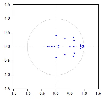
(5) According to the results in tables (4) and (5) and figure (2), It is clear that No root lies outside the unit circle, then VAR model satisfies the stability and consequently stationarity condition.
Figure (2). Inverse roots of AR characteristic polynomial
Table (1). Shows the results of model estimation and evaluation
Independent Variables
Dependent Variables
ER GF OI GDPS EXP IN EXS IMS FI II M2
ER(-1)
Parameter
estimation 1.291746 -3.359808 0.037610 0.005475 -20063.19 -163957.5 0.000769 2.186842 1946.338 -3543.093 13659.44 Standard
deviation (0.07291) (11.0445) (0.02569) (0.00393) (95828.4) (113146.) (0.00234) (1.30788) (1737.22) (3544.09) (6871.00) T statistic [ 17.7174] [-0.30421] [ 1.46389] [ 1.39230] [-0.20937] [-1.44908] [ 0.32833] [ 1.67204] [ 1.12037] [-0.99972] [ 1.98798] probability 0.0000 0.7632 0.1405 0.1636 0.8342 0.1475 0.7417 0.0929 0.2611 0.3170 0.0485
ER(-2)
Parameter
estimation -0.35058 -5.723954 -0.036043 -0.00533 29132.99 197231.4 -0.000873 -2.412683 1281.740 159.5519 -13933.86 Standard
Independent Variables
Dependent Variables
ER GF OI GDPS EXP IN EXS IMS FI II M2
T statistic [-4.74721] [-0.51166] [-1.38502] [-1.33798] [ 0.30014] [ 1.72094] [-0.36773] [-1.82121] [ 0.72841] [ 0.04445] [-2.00207] probability 0.0000 0.6123 0.1691 0.1777 0.7641 0.0855 0.7122 0.0686 0.4650 0.9613 0.0433
GF(-1)
Parameter
estimation -0.000285 0.614349 6.47E-05 -1.27E-05 -1469.215 -1755.393 1.16E-05 0.003263 7.097300 -34.301 -44.234 Standard
deviation (0.00057) (0.08571) (0.00020) (3.1E-05) (743.697) (878.094) (1.8E-05) (0.01015) (13.4821) (27.5046) (53.3239) T statistic [-0.50295] [ 7.16750] [ 0.32440] [-0.41634] [-1.97556] [-1.99910] [ 0.63596] [ 0.32144] [ 0.52642] [-1.24710] [-0.82953] probability 0.1341 0.0495 0.0607 0.1232 0.3849 0.5841 0.7840 0.3684 0.8188 0.4000 0.8040
GF(-2)
Parameter
estimation -0.000339 0.218795 2.97E-05 1.12E-05 1579.646 2066.176 -1.86E-05 -0.003121 30.40652 0.373897 89.19958 Standard
deviation (0.00057) (0.08699) (0.00020) (3.1E-05) (754.759) (891.155) (1.8E-05) (0.01030) (13.6826) (27.9138) (54.1170) T statistic [-0.58997] [ 2.51523] [ 0.14689] [ 0.36003] [ 2.09292] [ 2.31854] [-1.00751] [-0.30302] [ 2.22227] [ 0.01339] [ 1.64827] probability 0.3524 0.5835 0.8149 0.4164 0.5258 0.8128 0.2786 0.3798 0.8547 0.7415 0.5678
OI(-1)
Parameter
estimation -0.423735 -10.22577 1.488916 0.019160 147402.4 212580.9 0.019734 6.939136 4517.772 -12075.02 -11745.15 Standard
deviation (0.20813) (31.5289) (0.07334) (0.01123) (273563.) (323000.) (0.00669) (3.73364) (4959.27) (10117.4) (19614.7) T statistic [-2.03589] [-0.32433] [ 20.3011] [ 1.70675] [ 0.53882] [ 0.65815] [ 2.95070] [ 1.85855] [ 0.91097] [-1.19350] [-0.59879] probability 0.2082 0.6328 0.1761 0.8915 0.4852 0.3271 0.0000 0.4550 0.7520 0.3643 0.6180
OI(-2)
Parameter
estimation 0.499517 49.55186 -0.603835 -0.024738 125033.6 391844.5 -0.000925 -4.639323 -6680.866 19601.48 28321.38 Standard
deviation (0.24478) (37.0809) (0.08626) (0.01320) (321735.) (379878.) (0.00787) (4.39111) (5832.57) (11899.0) (23068.8) T statistic [ 2.04065] [ 1.33632] [-7.00043] [-1.87363] [ 0.38862] [ 1.03150] [-0.11758] [-1.05653] [-1.14544] [ 1.64733] [ 1.22769] probability 0.6075 0.9477 0.8536 0.6356 0.9366 0.8895 0.5141 0.5907 0.6089 0.7380 0.9245
GDPS(-1)
Parameter
estimation 1.503959 -308.6249 -1.055385 0.845137 1092146. 1753314. 0.009770 -26.49939 15972.33 24823.64 249914.3 Standard
deviation (1.98895) (301.296) (0.70087) (0.10728) (2614218) (3086645) (0.06391) (35.6793) (47391.8) (96683.4) (187442.) T statistic [ 0.75616] [-1.02432] [-1.50583] [ 7.87782] [ 0.41777] [ 0.56803] [ 0.15287] [-0.74271] [ 0.33703] [ 0.25675] [ 1.33329] probability 0.0015 0.6907 0.7261 0.3334 0.2507 0.2376 0.7508 0.5042 0.0000 0.5826 0.4479
GDPS(-2)
Parameter
estimation -2.908026 282.8078 0.421076 -0.108614 -21436.69 34403.71 -0.019947 -12.9734 -15893.86 27680.25 -99876.79 Standard
deviation (1.86583) (282.644) (0.65748) (0.10064) (2452385) (2895566) (0.05996) (33.4706) (44458.0) (90698.2) (175839.) T statistic [-1.55857] [ 1.00058] [ 0.64044] [-1.07924] [-0.00874] [ 0.01188] [-0.33270] [-0.38761] [-0.35750] [ 0.30519] [-0.56800] probability 0.0070 0.6718 0.7208 0.4119 0.3903 0.3761 0.9919 0.2974 0.4803 0.6344 0.5583
EXP (-1)
Parameter
estimation -2.46E-07 4.91E-05 1.09E-07 -1.37E-08 0.189673 -0.141078 -1.46E-09 -2.69E-06 0.000904 -0.006797 -0.003586 Standard
deviation (1.7E-07) (2.5E-05) (5.9E-08) (9.0E-09) (0.21822) (0.25766) (5.3E-09) (3.0E-06) (0.00396) (0.00807) (0.01565) T statistic [-1.47888] [ 1.95301] [ 1.86146] [-1.53201] [ 0.86918] [-0.54754] [-0.27321] [-0.90165] [ 0.22859] [-0.84220] [-0.22919] probability 0.4607 0.3058 0.1331 0.0000 0.6762 0.5701 0.8780 0.4579 0.7354 0.7952 0.1864
Independent Variables
Dependent Variables
ER GF OI GDPS EXP IN EXS IMS FI II M2
Parameter
estimation 1.66E-07 -1.41E-05 1.21E-08 7.36E-09 0.138564 -0.061063 5.76E-09 2.57E-06 0.000725 -0.002719 0.009653 Standard
deviation (1.7E-07) (2.5E-05) (5.9E-08) (9.0E-09) (0.21838) (0.25785) (5.3E-09) (3.0E-06) (0.00396) (0.00808) (0.01566) T statistic [ 0.99699] [-0.55975] [ 0.20686] [ 0.82127] [ 0.63450] [-0.23682] [ 1.07866] [ 0.86284] [ 0.18317] [-0.33667] [ 0.61649] probability 0.1208 0.3156 0.5209 0.2790 0.9930 0.9905 0.7385 0.6975 0.7198 0.7594 0.5701
IN(-1)
Parameter
estimation 1.42E-07 -3.58E-05 -1.02E-07 1.45E-08 0.407428 0.720724 1.18E-10 2.51E-06 -0.000717 0.005372 0.010562 Standard
deviation (1.4E-07) (2.1E-05) (4.8E-08) (7.4E-09) (0.17952) (0.21196) (4.4E-09) (2.5E-06) (0.00325) (0.00664) (0.01287) T statistic [ 1.03726] [-1.73116] [-2.12009] [ 1.97009] [ 2.26956] [ 3.40029] [ 0.02690] [ 1.02437] [-0.22035] [ 0.80913] [ 0.82053] probability 0.6125 0.0000 0.7432 0.6754 0.0484 0.0458 0.5234 0.7463 0.5974 0.2112 0.4048
IN(-2)
Parameter
estimation -1.39E-07 7.29E-06 -3.27E-08 -6.05E-09 -0.235336 -0.131785 -4.16E-09 -1.77E-06 -0.001372 -0.00074 -0.015643 Standard
deviation (1.4E-07) (2.1E-05) (4.9E-08) (7.6E-09) (0.18430) (0.21761) (4.5E-09) (2.5E-06) (0.00334) (0.00682) (0.01321) T statistic [-0.98796] [ 0.34343] [-0.66224] [-0.80055] [-1.27692] [-0.60561] [-0.92355] [-0.70512] [-0.41074] [-0.10858] [-1.18379] probability 0.4744 0.0106 0.8407 0.7347 0.0365 0.0206 0.3106 0.7785 0.0254 0.9762 0.1183
EXS(-1)
Parameter
estimation -4.467483 253.2506 1.665415 -0.026209 -3191803 -5292199 0.634055 -46.24675 26077.56 -152482.9 -168245.3 Standard
deviation (3.47875) (526.978) (1.22584) (0.18764) (4572362) (5398653) (0.11178) (62.4045) (82889.9) (169103.) (327843.) T statistic [-1.28422] [ 0.48057] [ 1.35859] [-0.13968] [-0.69806] [-0.98028] [ 5.67215] [-0.74108] [ 0.31460] [-0.90172] [-0.51319] probability 0.0661 0.9196 0.8552 0.5995 0.7304 0.5880 0.0765 0.8445 0.7785 0.0000 0.6853
EXS(-2)
Parameter
estimation 1.333305 43.76877 0.263427 0.079584 -341863.7 -704813.2 0.068175 32.53676 -39725.97 -50657.17 -52714.05 Standard
deviation (3.26926) (495.242) (1.15202) (0.17634) (4297005) (5073535) (0.10505) (58.6463) (77898.1) (158919.) (308100.) T statistic [ 0.40783] [ 0.08838] [ 0.22866] [ 0.45132] [-0.07956] [-0.13892] [ 0.64896] [ 0.55480] [-0.50997] [-0.31876] [-0.17109] probability 0.4020 0.4593 0.9348 0.7519 0.5324 0.3556 0.0796 0.9488 0.0075 0.0050 0.7312
IMS(-1)
Parameter
estimation -0.003556 0.370529 0.000534 -0.000259 2327.723 4248.334 8.02E-05 0.927196 -161.0082 -69.77312 -747.8715 Standard
deviation (0.00726) (1.09974) (0.00256) (0.00039) (9541.94) (11266.3) (0.00023) (0.13023) (172.981) (352.896) (684.167) T statistic [-0.48984] [ 0.33693] [ 0.20891] [-0.66270] [ 0.24395] [ 0.37708] [ 0.34380] [ 7.11967] [-0.93079] [-0.19772] [-1.09311] probability 0.6434 0.7394 0.8423 0.5091 0.8073 0.7062 0.7301 0.0000 0.3505 0.8402 0.2826
IMS(-2)
Parameter
estimation 0.005091 -0.266722 -0.001153 -4.03E-05 -528.9502 -1511.434 -0.000109 -0.077801 127.9697 91.78788 645.5435 Standard
deviation (0.00710) (1.07602) (0.00250) (0.00038) (9336.17) (11023.3) (0.00023) (0.12742) (169.250) (345.286) (669.413) T statistic [ 0.71672] [-0.24788] [-0.46059] [-0.10507] [-0.05666] [-0.13711] [-0.47539] [-0.61058] [ 0.75610] [ 0.26583] [ 0.96434] probability 0.4884 0.8071 0.6507 0.9130 0.9548 0.8910 0.6334 0.5428 0.4482 0.7876 0.3427
FI(-1)
Parameter
estimation -1.22E-05 0.000244 -2.92E-07 -1.93E-07 -5.425811 -6.58571 -3.58E-08 4.55E-05 0.849608 0.100138 -0.318125 Standard
Independent Variables
Dependent Variables
ER GF OI GDPS EXP IN EXS IMS FI II M2
T statistic [-3.40458] [ 0.44844] [-0.23076] [-0.99858] [-1.14919] [-1.18137] [-0.31019] [ 0.70534] [ 9.92627] [ 0.57348] [-0.93972] probability 0.2944 0.0820 0.0332 0.0479 0.0234 0.0007 0.9785 0.3056 0.8252 0.4181 0.4057
FI(-2)
Parameter
estimation 9.89E-06 -0.000241 2.96E-07 1.56E-07 3.820537 4.648070 -1.20E-09 -6.50E-05 -0.05567 -0.082102 -0.127953 Standard
deviation (3.4E-06) (0.00051) (1.2E-06) (1.8E-07) (4.44647) (5.25001) (1.1E-07) (6.1E-05) (0.08061) (0.16445) (0.31882) T statistic [ 2.92342] [-0.46985] [ 0.24810] [ 0.85266] [ 0.85923] [ 0.88534] [-0.01107] [-1.07092] [-0.69063] [-0.49926] [-0.40134] probability 0.3559 0.7402 0.4903 0.4282 0.2018 0.5449 0.3536 0.4719 0.6806 0.9069 0.2543
II(-1)
Parameter
estimation -3.33E-06 3.04E-05 1.29E-07 -5.02E-08 -0.787149 -1.460919 -9.85E-08 -5.68E-06 -0.011626 1.095319 0.058161 Standard
deviation (1.7E-06) (0.00026) (6.1E-07) (9.4E-08) (2.28365) (2.69634) (5.6E-08) (3.1E-05) (0.04140) (0.08446) (0.16374) T statistic [-1.91478] [ 0.11557] [ 0.21116] [-0.53584] [-0.34469] [-0.54182] [-1.76390] [-0.18221] [-0.28084] [ 12.9688] [ 0.35520] probability 0.5886 0.8565 0.6787 0.0638 0.0031 0.0032 0.4005 0.3028 0.9558 0.4856 0.0000
II(-2)
Parameter
estimation 1.60E-06 -0.000202 -6.69E-08 3.12E-08 1.456583 2.545098 9.96E-08 -2.40E-06 0.112769 -0.242103 0.064677 Standard
deviation (1.8E-06) (0.00027) (6.3E-07) (9.6E-08) (2.33250) (2.75401) (5.7E-08) (3.2E-05) (0.04228) (0.08626) (0.16724) T statistic [ 0.90172] [-0.75016] [-0.10699] [ 0.32614] [ 0.62447] [ 0.92414] [ 1.74602] [-0.07526] [ 2.66692] [-2.80653] [ 0.38673] probability 0.8260 0.8178 0.7815 0.0093 0.0026 0.0037 0.1862 0.1324 0.3237 0.9483 0.4331
M2(-1)
Parameter
estimation 4.38E-07 2.89E-05 -1.27E-07 -9.64E-08 -3.73872 -4.406125 -2.58E-08 -1.74E-05 0.001236 0.032910 0.880834 Standard
deviation (9.6E-07) (0.00015) (3.4E-07) (5.2E-08) (1.26206) (1.49013) (3.1E-08) (1.7E-05) (0.02288) (0.04668) (0.09049) T statistic [ 0.45619] [ 0.19865] [-0.37644] [-1.86203] [-2.96240] [-2.95687] [-0.83618] [-1.00937] [ 0.05404] [ 0.70508] [ 9.73394] probability 0.0433 0.7442 0.0000 0.0869 0.5901 0.5105 0.0031 0.0625 0.3607 0.2310 0.5517
M2(-2)
Parameter
estimation 2.55E-07 3.07E-05 8.34E-08 1.31E-07 3.682520 4.203941 3.94E-08 2.49E-05 -0.021778 -0.003233 0.072087 Standard
deviation (9.3E-07) (0.00014) (3.3E-07) (5.0E-08) (1.22302) (1.44404) (3.0E-08) (1.7E-05) (0.02217) (0.04523) (0.08769) T statistic [ 0.27377] [ 0.21801] [ 0.25433] [ 2.60267] [ 3.01100] [ 2.91124] [ 1.31678] [ 1.48951] [-0.98225] [-0.07147] [ 0.82204] probability 0.0481 0.1761 0.0000 0.0587 0.6976 0.3025 0.9062 0.2937 0.2499 0.0968 0.2349
C
Parameter
estimation 100.5544 12748.07 6.684152 2.581223 -20724629 -68251825 0.143767 847.8597 -4394116 4727355. 98509.20 Standard
deviation (39.5085) (5984.93) (13.9220) (2.13102) (5.2E+07) (6.1E+07) (1.26954) (708.732) (941387.) (1920513) (3723342) T statistic [ 2.54514] [ 2.13003] [ 0.48011] [ 1.21126] [-0.39910] [-1.11317] [ 0.11324] [ 1.19630] [-4.66770] [ 2.46151] [ 0.02646] probability 0.0077 0.0344 0.6673 0.2140 0.6899 0.2658 0.9096 0.2378 0.0000 0.0139 0.9072
R-squared 0.988381 0.993980 0.979363 0.957775 0.514482 0.598661 0.966681 0.969914 0.893609 0.971244 0.998694
Adj.
R-squared 0.986515 0.993013 0.976049 0.950994 0.436516 0.534212 0.961330 0.965083 0.876524 0.966627 0.998484
Log
likelihood -615.4898 -1418.767 -448.6027 -148.3032 -2869.708 -2896.288 -65.43179 -1077.404 -2228.065 -2342.144 -2448.068
Akaike AIC 7.981122 18.02209 5.895033 2.141290 36.15886 36.49109 1.105397 13.75505 28.13831 29.56430 30.88836
Table (2). VAR Lag Order Selection Criteria for Endogenous variables ER, EXP, EXS, FI, GDPS, GF, II, IMS, IN, M2 and OI
Lag LogL
LR FPE
AIC SC
HQ
0 -17610.44
NA 6.78e+85
228.8499 229.0668
228.9380
1 -15808.59
3322.900 2.25e+76
207.0206
209.6237* 208.0780*
2
-15678.75
220.8856* 2.05e+76*
206.9059*
211.8952 208.9325
3 -15586.42
143.8980 3.15e+76
207.2782 214.6536
210.2741
4 -15492.15
133.4418 4.98e+76
207.6254 217.3870
211.5905
5 -15386.24
134.8007 7.33e+76
207.8213 219.9691
212.7557
6 -15274.37
126.4020 1.11e+77
207.9398 222.4738
213.8435
7 -15157.55
115.2953 1.84e+77
207.9942 224.9144
214.8671
8 -14999.01
133.8379 2.19e+77
207.5066 226.8129
215.3488
* indicates lag order selected by the criterion: LR: sequential modified LR test statistic (each test at 5% level)
FPE: Final prediction error, AIC: Akaike information criterion, SC: Schwarz information criterion and HQ: Hannan-Quinn information criterion.
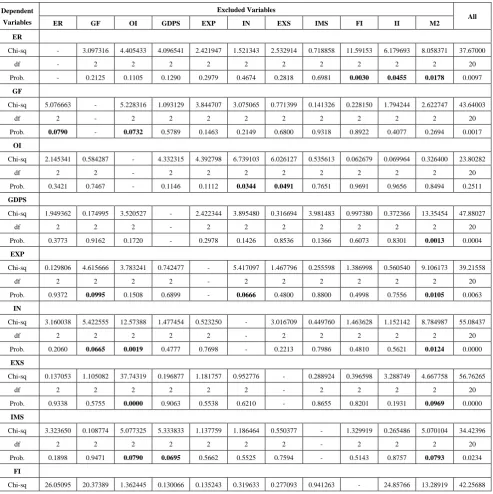
Table (3). VAR Granger Causality/Block Exogeneity Wald Tests
Dependent
Variables
Excluded Variables
All
ER GF OI GDPS EXP IN EXS IMS FI II M2
ER
Chi-sq - 3.097316 4.405433 4.096541 2.421947 1.521343 2.532914 0.718858 11.59153 6.179693 8.058371 37.67000
df - 2 2 2 2 2 2 2 2 2 2 20
Prob. - 0.2125 0.1105 0.1290 0.2979 0.4674 0.2818 0.6981 0.0030 0.0455 0.0178 0.0097
GF
Chi-sq 5.076663 - 5.228316 1.093129 3.844707 3.075065 0.771399 0.141326 0.228150 1.794244 2.622747 43.64003
df 2 - 2 2 2 2 2 2 2 2 2 20
Prob. 0.0790 - 0.0732 0.5789 0.1463 0.2149 0.6800 0.9318 0.8922 0.4077 0.2694 0.0017
OI
Chi-sq 2.145341 0.584287 - 4.332315 4.392798 6.739103 6.026127 0.535613 0.062679 0.069964 0.326400 23.80282
df 2 2 - 2 2 2 2 2 2 2 2 20
Prob. 0.3421 0.7467 - 0.1146 0.1112 0.0344 0.0491 0.7651 0.9691 0.9656 0.8494 0.2511
GDPS
Chi-sq 1.949362 0.174995 3.520527 - 2.422344 3.895480 0.316694 3.981483 0.997380 0.372366 13.35454 47.88027
df 2 2 2 - 2 2 2 2 2 2 2 20
Prob. 0.3773 0.9162 0.1720 - 0.2978 0.1426 0.8536 0.1366 0.6073 0.8301 0.0013 0.0004
EXP
Chi-sq 0.129806 4.615666 3.783241 0.742477 - 5.417097 1.467796 0.255598 1.386998 0.560540 9.106173 39.21558
df 2 2 2 2 - 2 2 2 2 2 2 20
Prob. 0.9372 0.0995 0.1508 0.6899 - 0.0666 0.4800 0.8800 0.4998 0.7556 0.0105 0.0063
IN
Chi-sq 3.160038 5.422555 12.57388 1.477454 0.523250 - 3.016709 0.449760 1.463628 1.152142 8.784987 55.08437
df 2 2 2 2 2 - 2 2 2 2 2 20
Prob. 0.2060 0.0665 0.0019 0.4777 0.7698 - 0.2213 0.7986 0.4810 0.5621 0.0124 0.0000
EXS
Chi-sq 0.137053 1.105082 37.74319 0.196877 1.181757 0.952776 - 0.288924 0.396598 3.288749 4.667758 56.76265
df 2 2 2 2 2 2 - 2 2 2 2 20
Prob. 0.9338 0.5755 0.0000 0.9063 0.5538 0.6210 - 0.8655 0.8201 0.1931 0.0969 0.0000
IMS
Chi-sq 3.323650 0.108774 5.077325 5.333833 1.137759 1.186464 0.550377 - 1.329919 0.265486 5.070104 34.42396
df 2 2 2 2 2 2 2 - 2 2 2 20
Prob. 0.1898 0.9471 0.0790 0.0695 0.5662 0.5525 0.7594 - 0.5143 0.8757 0.0793 0.0234
FI
Dependent
Variables
Excluded Variables
All
ER GF OI GDPS EXP IN EXS IMS FI II M2
df 2 2 2 2 2 2 2 2 - 2 2 20
Prob. 0.0000 0.0000 0.5060 0.9370 0.9346 0.8523 0.8706 0.6246 - 0.0000 0.0013 0.0026
II
Chi-sq 7.226421 4.383645 3.043823 1.310663 1.195673 0.689328 3.446200 0.086531 0.328982 - 6.218307 20.56340
df 2 2 2 2 2 2 2 2 2 - 2 20
Prob. 0.0270 0.1117 0.2183 0.5193 0.5500 0.7085 0.1785 0.9577 0.8483 - 0.0446 0.4232
M2
Chi-sq 4.116843 3.435801 2.621214 3.391340 0.380059 1.589727 1.086174 1.209556 6.570115 2.179424 - 35.37901
df 2 2 2 2 2 2 2 2 2 2 - 20
Prob. 0.1277 0.1794 0.2697 0.1835 0.8269 0.4516 0.5810 0.5462 0.0374 0.3363 - 0.0182
Table (4). Roots of Characteristic Polynomial for Exogenous variables C and Endogenous variablesER, GF, OI, GDPS, EXP, IN, EXS, IMS, FI, II and M2 with Lag specification: 1 2
Modulus Root
0.992161 0.992161
0.972620 0.971990 - 0.034996i
0.972620 0.971990 + 0.034996i
0.887163 0.885611 - 0.052456i
0.887163 0.885611 + 0.052456i
0.885879 0.885879
0.716361 0.630399 - 0.340249i
0.716361 0.630399 + 0.340249i
0.695934 0.655871 - 0.232717i
0.695934 0.655871 + 0.232717i
0.644114 0.644114
0.510897 0.510897
0.433906 0.326616 - 0.285650i
0.433906 0.326616 + 0.285650i
0.396172 0.016430 - 0.395831i
0.396172 0.016430 + 0.395831i
0.287712 -0.287712
0.227214 -0.227214
0.132879 -0.132879
0.120371 0.113804 - 0.039217i
0.120371 0.113804 + 0.039217i
0.049131 -0.049131
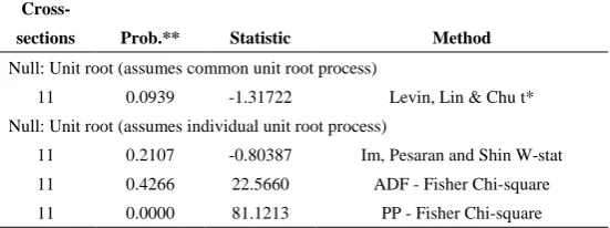
Table (5). Group unit root test: Summary for Series: ER, EXP, EXS, FI, GDPS, GF, II, IMS, IN, M2 and OI with lag length selection based on SIC from 0 to 13
Cross-
Method Statistic
Prob.** sections
Null: Unit root (assumes common unit root process)
Levin, Lin & Chu t* -1.31722
0.0939 11
Null: Unit root (assumes individual unit root process)
Im, Pesaran and Shin W-stat -0.80387
0.2107 11
ADF - Fisher Chi-square 22.5660
0.4266 11
PP - Fisher Chi-square 81.1213
4. Principal Component Analysis
For the purpose of policy-making and prioritization for economy of Iraq, principal component analysis is used. By using Kaiser criterion, we have three eigenvalues greater than one 6.084415, 2.18072 and 1.210415, so we have three factors. These factors contain 86.13% of information. The corresponding information for each factor taken as a percentage (86.13% will be treat as total information; by meaning that without losing a significant part of the original information) is as follows respectively, 64.2%, 23% and 12.8%.
The factors are,
(1) The first factor contains; Exchange Rate in market price (ER) variable (with a percentage of 17.2% (based on the information contained in the factor only) and 11% (based on all information included in the analysis), Exports (EX) variable (with a percentage of 20% (based on the information contained in the factor only) and 12.8% (based on all information included in the analysis), Gross Foreign Assets of CBI (GF) variable (with a percentage of 21.6% (based on the information contained in the factor only) and 13.9% (based on all information included in the analysis), Imports (IM) variable (with a percentage of 20.9% (based on the information contained in the factor only) and 13.5% (based on all information included in the analysis) and Broad Money (M2) variable (with a percentage of 20.3% (based on the information contained in the factor only) and 13% (based on all information included in the analysis).
(2) The second factor contains; Foreign Investment (FI) variable (with a percentage of 28.4% (based on the information contained in the factor only) and 6.6% (based on all information included in the analysis), Gross Domestic Product In Constant Price (2007=100) (GDP) variable (with a percentage of 18.2% (based on the information contained in the factor only) and 4.2% (based on all information included in the analysis), Iraqi Investment (II) variable (with a percentage of 28.9% (based on the information contained in the factor only) and 6.6% (based on all
information included in the analysis) and Oil price (OI) variable (with a percentage of 24.5% (based on the information contained in the factor only) and 5.6% (based on all information included in the analysis).
(3) The third factor contains; Expenses (EXP) variable (with a percentage of 53.3% (based on the information contained in the factor only) and 6.8% (based on all information included in the analysis) and Income (IN) variable (with a percentage of 46.7% (based on the information contained in the factor only) and 6% (based on all information included in the analysis).
Based on the above results, all plans, policies and programs of economic and development in Iraq must be made according to the effects of factors and consequently variables under consideration.
5. Summary
Most important eleven variables in Iraqi economy have been considered. Some of these variables have been compiled on an annual basis, while the other variables were compiled on a monthly basis. To unify these basis, the monthly values of these variables are simulated. VAR model is estimated and all related tests and indicators are obtained. The VAR model presented here has become ready for Iraqi economy explanation and forecasting. principal component analysis is used for the purpose of policy-making and prioritization for economy of Iraq. According to the effects of factors and consequently variables under consideration, plans and policies of economic and development in Iraq must be done.
ACKNOWLEDGMENTS
Appendix
Table (1). Data of variables under consideration, Foreign Investment (FI), Iraqi Investment (II), Imports (IM), Exports (EX), Expenses (EXP), Income (IN), Broad Money (M2), Oil price (OI), Gross Domestic Product In Constant Price (2007=100) (GDP), Gross Foreign Assets of CBI (GF) and Exchange Rate in market price (ER)
DATE FI II IMS EXS EXP IN M2 OI GDPS GF ER
1/31/2004 567,602 1,560,816 264.0679 0.23117 468,749 1,119,448 7,445,000 26.39 1.496749701 1,569.12 1,476
2/29/2004 567,602 1,563,185 526.3 0.470993 1,119,353 1,886,653 7,671,000 26.48 2.938197214 2,071.58 1,409
3/31/2004 567,602 1,230,167 786.7591 0.71922 1,920,634 3,242,379 7,899,000 27.46 4.325647332 1,828.77 1,422
4/30/2004 637,627 1,249,460 1045.506 0.975607 2,618,212 4,145,310 8,261,000 26.70 5.66039111 2,257.64 1,442
5/31/2004 637,627 1,278,742 1302.601 1.239909 3,488,315 4,960,940 8,502,000 30.29 6.943705872 2,842.47 1,462
6/30/2004 999,745 1,413,113 1558.102 1.511883 15,097,975 13,218,342 9,147,000 30.74 8.176855202 3,193.15 1,460
7/31/2004 999,779 989,967 1812.063 1.791289 16,540,405 21,085,926 9,367,000 31.28 9.361088953 4,413.70 1,463
8/31/2004 1,025,992 1,310,011 2064.541 2.077885 18,797,954 23,781,490 9,705,000 34.01 10.49764324 4,462.33 1,463
9/30/2004 1,028,912 1,559,589 2315.587 2.371436 20,869,089 27,876,535 9,775,000 34.83 11.58774044 5,095.21 1,463
10/31/2004 1,028,912 1,234,057 2565.252 2.671703 24,374,839 33,274,185 9,588,000 37.00 12.6325892 4,733.56 1,463
11/30/2004 1,028,912 1,292,994 2813.586 2.978453 26,800,967 40,022,031 9,885,000 39.14 13.63338443 5,679.45 1,463
12/31/2004 1,055,556 1,076,225 3060.636 3.291452 32,117,491 32,982,739 12,254,000 30.72 14.59130731 6,924.08 1,462
1/31/2005 1,055,557 890,114 1399.721 1.298793 1,010,030 4,965,739 12,474,000 27.79 6.811261203 8,286.93 1,457
2/28/2005 1,133,741 766,734 1503.275 1.415634 2,527,842 4,132,869 12,899,000 28.44 7.195874147 8,976.77 1,461
3/31/2005 1,228,687 1,040,098 1606.342 1.534475 4,757,612 7,498,260 13,650,000 38.49 7.563176768 9,332.69 1,469
4/30/2005 1,291,209 1,390,243 1708.939 1.655234 6,332,496 11,027,989 13,732,000 40.51 7.913663732 8,324.88 1,474
5/31/2005 1,367,018 1,784,801 1811.083 1.77783 7,432,887 14,014,371 13,888,000 42.28 8.247823676 9,274.78 1,473
6/30/2005 1,383,975 1,775,045 1912.789 1.902182 10,352,309 18,592,689 13,792,000 41.65 8.5661392 8,893.86 1,468
7/31/2005 1,397,883 1,160,531 2014.072 2.028211 13,160,137 21,806,294 14,036,000 46.82 8.869086873 8,904.18 1,475
8/31/2005 1,422,586 793,640 2114.946 2.155837 15,705,267 26,618,844 13,278,000 51.65 9.157137232 8,407.10 1,480
9/30/2005 1,436,480 927,031 2215.427 2.284981 18,229,751 30,285,106 13,138,000 55.40 9.430754779 9,236.80 1,481
10/31/2005 1,446,933 1,069,174 2315.525 2.415566 20,267,030 34,618,385 14,051,000 53.67 9.690397985 10,033.20 1,476
11/30/2005 1,456,790 1,315,269 2415.254 2.547512 22,791,497 37,805,783 13,272,000 48.04 9.936519288 10,564.12 1,477
12/31/2005 1,573,156 1,406,780 2514.626 2.680744 26,375,175 40,502,890 14,684,000 46.07 10.16956509 12,001.15 1,478
1/31/2006 1,632,947 1,466,189 1521.44 2.002157 2,087,710 2,450,635 15,267,000 45.62 8.35484398 12,414.17 1,482
2/28/2006 1,687,586 1,668,324 1578.887 2.098577 4,096,114 5,198,145 15,826,000 50.54 8.522270851 12,801.02 1,480
3/31/2006 1,750,016 1,468,759 1636.144 2.195749 8,110,930 8,841,160 16,701,000 50.86 8.680231169 13,209.86 1,480
4/30/2006 1,741,213 1,329,528 1693.215 2.293619 11,358,817 12,552,373 16,842,000 54.43 8.829064494 13,567.91 1,481
5/31/2006 1,894,425 915,613 1750.104 2.392136 14,333,493 17,201,883 17,128,000 59.85 8.969105537 13,460.99 1,485
6/30/2006 1,919,979 712,079 1806.817 2.491245 16,459,986 21,453,026 17,486,000 59.91 9.100684156 12,903.57 1,485
7/31/2006 1,929,041 929,099 1863.357 2.590897 19,257,550 26,869,120 18,820,000 62.13 9.224125357 13,032.44 1,486
8/31/2006 1,983,459 1,155,442 1919.727 2.691038 21,938,206 32,293,996 19,440,000 64.06 9.339749297 14,266.79 1,488
9/30/2006 1,952,560 1,543,771 1975.93 2.791618 24,742,634 36,980,609 19,145,000 59.37 9.44787128 14,579.62 1,488
10/31/2006 1,823,294 1,942,109 2031.969 2.892586 27,352,221 41,441,677 19,538,000 52.79 9.548801759 14,794.39 1,485
11/30/2006 1,804,268 2,114,544 2087.846 2.993892 30,206,873 45,047,874 19,658,000 49.12 9.642846338 13,951.09 1,463
12/31/2006 1,783,338 2,402,937 2143.563 3.095485 38,806,679 49,055,545 21,080,000 52.14 9.730305767 19,741.69 1,396
1/31/2007 1,798,914 2,771,767 1433.021 2.805965 1,350,445 3,093,583 18,329,063 50.15 8.994614893 19,283.59 1,318
2/28/2007 1,838,729 3,298,346 1469.121 2.895498 3,084,154 5,432,384 18,521,249 48.87 9.063528378 17,750.37 1,298
3/31/2007 1,898,701 3,234,100 1505.118 2.985153 4,946,238 8,930,537 18,677,529 50.56 9.127205416 18,051.47 1,290
4/30/2007 1,524,395 3,233,720 1541.012 3.074888 7,473,210 12,580,359 19,144,052 55.45 9.185903931 19,900.57 1,284
5/31/2007 1,986,318 3,792,123 1576.803 3.164662 11,251,064 16,466,089 18,147,866 57.39 9.239877397 20,642.57 1,274
6/30/2007 1,485,045 4,514,616 1612.49 3.254432 13,101,040 20,325,291 18,791,275 61.17 9.289374844 21,463.73 1,269
7/31/2007 1,528,639 4,667,253 1648.073 3.344158 16,008,157 24,745,620 19,577,348 64.76 9.334640852 23,783.24 1,260
8/31/2007 1,517,369 5,130,326 1683.55 3.433797 18,617,390 29,969,998 20,301,736 66.87 9.375915554 24,171.56 1,253
DATE FI II IMS EXS EXP IN M2 OI GDPS GF ER
10/31/2007 1,482,053 5,197,216 1754.182 3.612656 26,411,509 39,321,208 23,444,731 72.05 9.447429342 25,051.15 1,245
11/30/2007 1,553,761 4,663,392 1789.334 3.701794 28,960,902 44,846,186 23,522,876 78.11 9.478126457 27,102.67 1,240
12/31/2007 2,447,922 3,864,737 1824.372 3.790687 39,031,232 54,599,451 26,956,076 84.49 9.505748329 31,584.37 1,214
1/31/2008 1,540,911 3,028,832 2648.362 4.728656 1,607,046 2,573,093 27,037,186 83.86 9.963173793 31,912.70 1,225
2/29/2008 1,447,203 2,717,629 2697.939 4.836267 4,995,678 13,167,767 25,349,193 81.76 9.986298642 32,715.65 1,225
3/31/2008 1,559,650 2,237,622 2747.345 4.943434 7,975,770 19,855,874 25,910,917 92.19 10.00687806 34,734.32 1,222
4/30/2008 1,596,680 2,669,807 2796.573 5.050112 12,954,951 26,682,483 26,081,245 95.68 10.02512589 35,342.71 1,216
5/31/2008 1,583,147 2,612,633 2845.62 5.156254 17,400,673 36,912,497 26,580,025 104.28 10.04125132 38,554.72 1,212
6/30/2008 1,549,737 2,877,012 2894.48 5.261815 22,952,019 45,762,082 28,481,094 115.98 10.05545889 39,019.45 1,205
7/31/2008 1,334,443 3,020,477 2943.147 5.36675 27,721,807 54,976,044 29,825,484 123.73 10.06794851 40,184.50 1,202
8/31/2008 1,329,367 3,400,990 2991.615 5.471012 31,612,445 60,449,222 30,879,575 113.05 10.07891541 39,296.28 1,196
9/30/2008 1,381,991 3,895,030 3039.877 5.574559 38,556,973 67,230,278 32,536,077 101.74 10.08855019 44,522.79 1,188
10/31/2008 1,366,745 3,464,679 3087.927 5.677346 43,450,505 72,769,996 31,294,688 83.70 10.09703879 42,964.34 1,185
11/30/2008 1,331,321 3,566,555 3135.756 5.779329 49,385,768 76,498,131 33,579,985 59.03 10.10456252 45,768.93 1,183
12/31/2008 1,261,697 3,055,803 3183.358 5.880466 59,403,375 80,252,182 34,919,675 43.97 10.11129803 50,305.71 1,180
1/31/2009 1,239,949 2,685,415 3207.076 3.019878 2,129,132 2,584,767 36,057,912 34.88 10.35892081 46,636.80 1,178
2/28/2009 1,228,084 2,459,853 3253.853 3.070026 4,687,280 5,053,218 37,659,037 37.14 10.36472656 43,627.17 1,178
3/31/2009 1,257,846 3,152,044 3300.378 3.119683 7,573,558 8,285,472 36,973,388 37.83 10.3702393 41,885.24 1,178
4/30/2009 1,253,328 2,446,040 3346.643 3.168827 10,659,729 11,552,920 36,720,694 43.85 10.37562086 41,442.14 1,179
5/31/2009 1,265,963 2,671,634 3392.638 3.217438 14,480,889 15,577,385 36,957,496 48.93 10.38102829 40,895.15 1,187
6/30/2009 1,295,121 2,737,795 3438.352 3.265495 19,308,998 20,263,399 37,811,325 56.30 10.3866139 41,633.20 1,180
7/31/2009 1,325,976 2,517,368 3483.776 3.312979 23,562,094 25,317,228 38,806,875 64.49 10.39252525 43,422.63 1,184
8/31/2009 1,336,357 2,404,376 3528.898 3.359869 27,604,557 31,894,860 39,690,346 64.16 10.3989051 42,180.63 1,184
9/30/2009 1,342,040 2,911,827 3573.707 3.406145 33,073,579 39,251,341 42,982,641 68.16 10.40589148 40,136.72 1,183
10/31/2009 1,513,607 2,974,988 3618.193 3.451787 38,198,670 44,156,826 42,921,266 65.74 10.41361766 43,023.59 1,183
11/30/2009 1,528,246 2,975,291 3662.342 3.496777 43,521,533 49,350,292 43,813,715 71.50 10.42221214 45,002.51 1,183
12/31/2009 1,550,025 3,304,308 3706.143 3.541095 52,567,025 55,209,353 45,437,918 74.02 10.43179866 44,636.05 1,185
1/31/2010 1,537,010 6,158,947 3448.805 4.062145 3,861,589 5,028,681 46,211,046 73.37 10.95855232 45,478.66 1,185
2/28/2010 1,536,389 7,090,382 3488.417 4.110779 7,688,959 9,447,768 47,666,215 73.99 10.97106433 43,892.75 1,185
3/31/2010 1,361,809 9,304,441 3527.672 4.158587 11,624,023 16,583,140 49,264,741 72.98 10.984977 42,923.92 1,185
4/30/2010 1,413,430 9,142,084 3566.557 4.20555 15,931,096 23,322,826 51,224,102 76.46 11.00040022 43,410.69 1,185
5/31/2010 1,641,402 9,891,999 3605.061 4.251647 21,249,373.26 28,341,752 53,050,750 79.93 11.01743887 41,310.72 1,185
6/30/2010 1,613,288 8,706,263 3643.168 4.296857 26,691,602 34,339,563 55,851,298 73.32 11.03619283 42,431.47 1,185
7/31/2010 1,675,474 9,229,299 3680.866 4.341161 32,432,019 39,441,639 55,873,827 71.07 11.056757 42,821.02 1,185
8/31/2010 1,572,032 8,067,252 3718.14 4.384539 37,881,009 44,288,704 56,388,061 72.08 11.07922126 43,227.34 1,185
9/30/2010 1,692,920 8,465,120 3754.976 4.426971 42,410,560 51,082,931 56,213,464 71.65 11.10367052 46,178.48 1,185
10/31/2010 1,694,460 8,760,586 3791.359 4.468439 47,319,988 56,774,979 57,299,232 73.25 11.13018468 46,616.03 1,185
11/30/2010 1,544,722 8,962,474 3827.274 4.508922 51,839,037 62,377,046 58,201,459 77.59 11.15883865 47,591.58 1,185
12/31/2010 1,514,834 6,228,635 3862.704 4.548402 64,351,984 69,521,117 60,386,086 80.74 11.18970235 50,652.39 1,185
1/31/2011 1,511,243 5,581,601 3808.866 6.381708 3,583,740 7,337,215 60,808,829 86.44 11.64205631 51,467.61 1,185
2/28/2011 1,493,234 5,647,763 3842.496 6.433771 7,539,833 14,848,018 59,739,929 91.09 11.67885425 50,620.97 1,185
3/31/2011 1,508,885 5,794,005 3875.607 6.484362 12,735,146 24,046,963 58,452,768 97.75 11.71813095 50,403.93 1,185
4/30/2011 1,529,036 5,268,718 3908.18 6.533458 17,828,846 32,607,727 59,265,111 107.84 11.75993819 53,665.32 1,187
5/31/2011 1,506,485 5,167,941 3940.199 6.581033 22,951,921 42,576,070 59,602,270 114.77 11.80432259 54,331.59 1,196
6/30/2011 1,501,047 5,023,153 3971.646 6.627064 28,861,159 50,815,526 62,321,706 108.34 11.85132558 54,351.18 1,197
7/31/2011 1,461,013 5,310,130 4002.505 6.671526 35,791,501 59,239,035 64,438,666 105.32 11.90098341 53,521.14 1,197
8/31/2011 1,470,375 5,189,236 4032.756 6.714398 41,786,546 67,868,691 65,125,368 109.21 11.95332716 57,219.93 1,199
9/30/2011 1,471,031 5,100,354 4062.382 6.755655 46,753,668 76,201,593 65,110,706 104.71 12.0083827 56,915.67 1,200