http://www.gjaets.com (C) Global Journal of Advance Engineering Technology and Sciences
9
Global Journal of Advance Engineering Technology and Science
ISOLATED WORD SPEECH RECOGNITION SYSTEM USING
DYNAMIC TIME WARPING
Sapana Badawdiya*
1, Neha Sharma
2PG Scholar*
1, Asst. Professor
2, Electronics and Communication Engg. Deptt.
*
1,2Ujjain Engineering College ,Ujjain (M.P)
[email protected]
Abstract
Speech recognition is a multileveled pattern recognition task, in which acoustical signals are examined and structured into a hierarchy of sub word units (e.g., phonemes), words,phrases, and sentences. Each level may provide additional temporal constraints, e.g., known word pronunciations or legal word sequences, which can compensate for errors or uncertainties at lower levels. This hierarchy of constraints can best be exploited by combining decisions probabilistically at all lower levels, and making discrete decisions only at the highest level.Dynamic time warping is a unessential concept used primarily for applications where low computation is required. The paper describes a system based on dynamic programming concept[1]. The software was built using
Mat lab 8.01.
Index Terms--- Dynamic time warping, dynamic programming, Euclidiandistance. Speech recognition, Mel cepstrum , Mel frequency
1. Introduction
In speech recognition, the main goal of the feature extraction step is to compute a parsimonious sequence of feature vectors providing a compact representation of the given input signal. The feature extraction is usually performed in three stages. The first stage is called the speech analysis or the acoustic front end. It performs some kind of spectrum temporal analysis of the signal and generates raw features describing the envelope of the power spectrum of short speech intervals. The second stage compiles an extended feature vector composed of static and dynamic features. Finally, the last stage (which is not always present) transforms these extended feature vectors into more compact and robust vectors that are then supplied to the recognizer. Although there is no real consensus as to what the optimal feature sets should look like, one usually would like them to have the following properties: they should allow an automatic system to discriminate between different through similar sounding speech sounds, they should allow for the automatic creation of acoustic models for these sounds without the need for an excessive amount of training data, and they should exhibit statistics which are largely invariant cross speakers and speaking environment.
2.
Simple Model of Speech Production
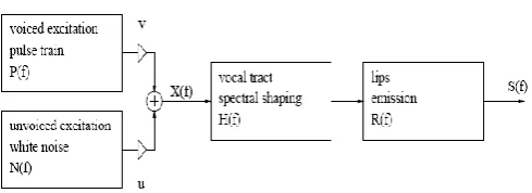
The production of speech can be separated into two parts: Producing the excitation signal and forming the spectral shape. Thus, we can draw a simplified model of speech production as shown below :Figure 1: A simple model of speech production
This model works as follows: Voiced excitation is modeled by a pulse generator which generates a pulse train (of triangle–shaped pulses) with its spectrum given by P (f). The unvoiced excitation is modeled by a white noise generator with spectrum N (f). To mix voiced and unvoiced excitation, one can adjust the signal amplitude of the impulse generator (v) and the noise. Thus from the above model we get :-
P(f) = Voiced excitation pulse train N(f)= Unvoiced excitation (white noise) H(f)= Transfer function of vocal tract R(f)= transfer function of lip emmision S(f)= Final voice signal
2.1 Human Speech Coefficients
The human ear does not show a linear
frequency resolution but builds several groups
of frequencies and integrates the spectral
energies within a given group. Furthermore,
the mid-frequency and bandwidth of these
groups are non–linearly distributed. The non–
linear warping of the frequency axis can be
modeled by the so–called Mel-scale[2]. Thehttp://www.gjaets.com (C) Global Journal of Advance Engineering Technology and Sciences
10
distributed along the Mel-scale. The so–called Mel–frequency f_ Mel can be computed from the frequency f as follows:
f_ Mel (f)=2595∙log10(1+f/(700 Hz))
(1)
The human ear has high frequency resolution in low–frequency parts of the spectrum and low frequency resolution in the high–frequency parts of the spectrum. The coefficients of the power spectrum [|V (n) |]^2 are now transformed to reflect the frequency resolution of the human ear.
2.2 Cepstrum Wise Coefficients
The direct computation of the power spectrum from the speech signal results in a spectrum containing “ripples” caused by the excitation spectrum X(f). Depending on the implementation of the acoustic preprocessing however, special transformations are used to separate the excitation spectrum X (f) from the spectral shaping of the vocal tract H (f). Thus, a smooth spectral shape (without the ripples), which represents H (f) can be estimated from the
S(f) = X(f)•H(f)•R(f)=H(f)•U(f)(2)
We can now transform the product of the spectral functions to a sum by taking the logarithm on both sides of the equation:
log10 [(S(f)] =log10[H(f)]∙[U(f)]=log10 [H(f)]
+log1o[U(f)]
(3)
This holds also for the absolute values of the power spectrum and also for their squares:
log10 [(|S (f)|2 ] =log10 [(|H (f)|2∙|U (f)|2]
=log10 [ |H (f)|2] +log10 [|U (f)|2] (4)
In figure 2 we see an example of the log power spectrum, which contains unwanted ripples caused by the excitation signal.
As we recall, it is necessary to compute the speech parameters in short time intervals to reflect the dynamic change of the speech signal. Typically, the spectral parameters of speech are estimated in time intervals of 10 ms[3]. First, we
have to sample and digitize the speech signal. Depending on the implementation, a sampling frequency f_s between 8 kHz and 16 kHz and usually a 16 bit quantization of the signal amplitude is used.After digitizing the analog speech signal, we get a series of speech samples s(k∙∆t) where ∆t = 1/f_s or, for easier notation, simply
s(k).s ̂(d)=[FT]^(-1) {log(|S(f)|^2 ) }
=[FT]^(-1) {log(|H(f)|^2 ) }+[FT]^(-1){log(|U(f)|^2 )}
(5)
Figure 2: Log power spectrum of the vowel /a: / (f_s = 11 kHz). The ripples in the spectrum are
caused by X (f)
The inverse Fourier transform brings us back to the time–domain (d is also called the delay or frequency), giving the so–called cepstrum (a reversed “spectrum”)[4]. The resulting cepstrum is
real–valued, since [|U(f)|]^2 and [|H(f)|]^2 are both real-valued and both are even: [|U(f)|]^2= [|U(-f)|]^2 and [|H([|U(-f)|]^2=[|H(-[|U(-f)|]^2. Applying the inverse DFT to the log power spectrum coefficients log[(|V (n)|)^2 ] yields:
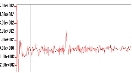
Figure 3: Cepstrum of the vowel /a: / (f_s = 11 kHz, N = 512). The ripples in the spectrum
result in a peak in the cepstrum
2.3 Mel Cepstrum
Now that we are familiar with the cepstrum transformation and cepstrumsmoothing, we will compute the Mel cepstrum commonly used in speech recognition. As stated above, for speech recognition, the Mel spectrum is used to reflect the perception characteristics of the human ear. In analogy to computing the cepstrum, we now take the logarithm of the Mel power spectrum given by :- 𝐺(𝑘) = ∑𝑁/2𝑛=0𝜂kn|𝑉(𝑛)|2 ; 𝑘 = 0,1,2 … … (6)
http://www.gjaets.com (C) Global Journal of Advance Engineering Technology and Sciences
11
are used in typical speech recognition systems. The restriction to the first Q coefficients reflects the low–pass filtering process as described above.
Since the Mel power spectrum is symmetric due to (6), the Fourier-Transform can be replaced by a simple cosine transform:
c(q) = ∑ log(G(k))
κ−1
k=0
∙ cos (πq(2k + 1) 2К ) ; q
= 0, 1, … , 𝒬 − 1
(7)
While successive coefficients G(k) of the Mel power spectrum are correlated, the Mel Frequency Cepstrum Coefficients (MFCC)[5] resulting from
the cosine transform (7) are decorrelated.
Figure 4: Mel cepstrum of an isolated word
Fig 5 Log power spectrum of word “HELLO”
Fig.6 Log energyspectrum of word “HELLO”
Fig.7 Log Mel power spectrum of word “HELLO”
3. Dynamic time warping
Our speech signal is represented by a series of feature vectors which are computed every 10 ms. A whole word will comprise dozens of those vectors, and we know that the number of vectors (the duration) of a word will depend on how fast a person is speaking. Therefore, our classification task is different from what we have learned before. In speech recognition, we have to classify not only single vectors, but sequences of vectors. Let’s assume we would want to recognize a few command words or digits. For an utterance of a word w which is T_X vectors long, we will get a sequence of vectors X ={x _0, x _1... x _(X-1)} from the acoustic preprocessing stage. What we need here is a way to compute a “distance” between this unknown sequence of vectors X and known sequences of vectors W _k={w _(k0,) w _(k1,) …,w _(kT_(W_k ) ) } which are prototypes for the words we want to recognize. Let our vocabulary (here: the set of classes Ω) contain V different words w_0,w_1,...w_(V-1). In analogy to the Nearest Neighbor classification task from section 3, we will allow a word w_v (here: class w_v∈Ω) to be represented by a set of prototypes W_(k,ω_v ),k=0,1,…,(K_(ω_v )-1) to reflect all the variations possible due to different pronunciation or even different speakers.
Fig 8: Possible assignment between vector pairs of X and W
3.1 Distance between Two Sequences of
Vectors
Classification of a spoken utterance would be easy if we had a good distance measure 𝐷(𝑋̃ , 𝑊̃ ) at hand (in the following, we will skip the additional indices for ease of notation). What should the properties of this distance measure be? The distance measure we need must:
http://www.gjaets.com (C) Global Journal of Advance Engineering Technology and Sciences
12
2. While computing the distance, find an optimal assignment between the individual feature vectors of 𝑋̃ and 𝑊̃
3. Compute a total distance out of the sum of distances between individual pairs of feature vectors of 𝑋̃ and 𝑊̃.
3.2 Comparing Sequences With Different
Lengths
The main problem is to find the optimal assignment between the individual vectors of 𝑋̃ and
𝑊̃. In Fig. 3.16 we can see two sequences 𝑋̃ and 𝑊̃ which consist of six and eight vectors, respectively. The sequence 𝑊̃ was rotated by 90 degrees, so the time index for this sequence runs from the bottom of the sequence to its top. The two sequences span a grid of possible assignments between the vectors. Each path through this grid (as the path shown in the figure) represents one possible assignment of the vector pairs. For example, the first vector of 𝑋̃ is assigned the first vector of 𝑊̃ , the second vector of 𝑋̃ is assigned to the second vector of 𝑊̃, and so on.
Fig. 9 shows as an example the following path 𝑃 given by the sequence of time index pairs of the vector sequences[6](or the grid point indices,
respectively):
P = {g1, g2, . . , gLp}
= {(0,0), (1,1), (2,2), (5,3)} (8)
The length 𝐿𝑃 of path 𝑃 is determined by
the maximum of the number of vectors contained in
𝑋̃ and𝑊̃ . The assignment between the time indices of 𝑊̃ and 𝑋̃ as given by 𝑃 can be interpreted as “time warping” between the time axes of 𝑊̃and 𝑋̃ . In our example, the vectors𝑥⃗2, 𝑥⃗3 and 𝑥⃗4were all
assigned to 𝑤⃗⃗⃗2, thus warping the duration of 𝑤⃗⃗⃗2 so that it lasts three time indices instead of one. By this kind of time warping, the different lengths of the vector sequences can be compensated.
For the given path 𝑃, the distance measure between the vector sequences can now be computed as the sum of the distances between the individual vectors. Let 𝑙 denote the sequence index of the grid points. Let 𝑑(𝑔𝑙) denote the vector distance 𝑑 (𝑥⃗2, 𝑤⃗⃗⃗𝑗) for the time indices 𝑖 and 𝑗 defined by the grid point 𝑔𝑙 = (𝑖, 𝑗) (the distance
𝑑 (𝑥⃗2, 𝑤⃗⃗⃗𝑗) could be the Euclidean distance from eq
(8). Then the overall distance can be computed as:
D(X̃, W̃ , P)
= ∑ d
LP
l=1
(gl) (9)
3.3 Finding the Optimal Path
As we stated above, once we have the path, computing the distance D is a simple task. How do we find it? The criterion of optimality we want to
use in searching the optimal path poptshould be to
minimize𝐷(𝑋̃, 𝑊̃ , 𝑃):
Popt
=arg
min
P {D(X̃, W̃ , P)} (10)
Fortunately, it is not necessary to compute all possible paths P and corresponding distances
𝐷(𝑋̃, 𝑊̃ , 𝑃)to find the optimum.
Out of the huge number of theoretically possible paths, only a fraction is reasonable for our purposes. We know that both sequences of vectors represent feature vectors measured in short time intervals. Therefore, we might want to restrict the time warping to reasonable boundaries: The first vectors of 𝑋̃and 𝑊̃ should be assigned to each other as well as their last vectors. For the time indices in between, we want to avoid any giant leap backward or forward in time, but want to restrict the time warping just to the “reuse” of the preceding vector(s) to locally warp the duration of a short segment of speech signal. With these restrictions, we can draw a diagram of possible “local” path alternatives[7] for one grid point and its possible
predecessors (of course, many other local path diagrams are possible):
Fig. 9: Local path alternatives for a grid point
Note that Fig. 9 does not show the possible extensions of the path from a given point but the possible predecessor paths for a given grid point. As we can see, a grid point (𝑖, 𝑗) can have the following predecessors:
1. (𝑖 − 1, 𝑗0): Keep the time index 𝑗 of 𝑋̃ while the time index of 𝑊̃ is incremented. 2. (𝑖 − 1, 𝑗 − 1): Both time indices of 𝑋̃ and
𝑊̃ are incremented.
http://www.gjaets.com (C) Global Journal of Advance Engineering Technology and Sciences
13
from (𝑖 − 1, 𝑗 − 1), the diagonal transition involves only the single vector distance at grid point (𝑖, 𝑗) as opposed to using the vertical or horizontal transition, where also the distances for the grid points (𝑖 − 1, 𝑗) or (𝑖, 𝑗 − 1) would have to be added. To compensate this effect, the local distance
𝑑( 𝑤⃗⃗⃗𝑖, 𝑥⃗𝑗) is added twice when using the diagonal
transition.
3.4Bellman’s Principle
[8]Now that we have defined the local path alternatives, we will use Bellman’s Principle to search the optimal path𝑃𝑜𝑝𝑡.Whenapplied to our problem the , Bellman’s Principle states the following:
If Popt is the optimal path through the matrix of grid points beginning at (0, 0) and ending at (TW−1, TX−1), and the grid point (i, j) is part of
path Popt, then the partial path from (0, 0) to (i, j) is
also part of Popt. From that, we can construct a way of iteratively finding our optimal path 𝑃𝑜𝑝𝑡 :
According to the local path alternatives diagram we chose, there are only three possible predecessor paths leading to a grid point(𝑖, 𝑗): The partial paths from (0, 0) to the grid points (𝑖 − 1, 𝑗), (𝑖 − 1, 𝑗 −
1) 𝑎𝑛𝑑 (𝑖, 𝑗 − 1)).
Let’s assume we would know the optimal paths (and therefore the accumulated distance 𝛿(. ) along that paths) leading from (0, 0) to these grid points. All these path hypotheses are possible predecessor paths for the optimal path leading from
(0, 0)to(𝑖, 𝑗).
Then we can find the (globally) optimal path from (0, 0) to grid point (𝑖, 𝑗) by selecting exactly the one path hypothesis among our alternatives which minimizes the accumulated distance 𝛿(𝑖, 𝑗) of the resulting path from
(0, 0)to(𝑖, 𝑗).
The optimization we have to perform is as follows:
𝛿(𝑖, 𝑗) =min{
𝛿(𝑖, 𝑗 − 1) + 𝑑(𝑤⃗⃗⃗𝑖, 𝑥⃗𝑗)
𝛿(𝑖 − 1, 𝑗 − 1) + 2 ∙ 𝑑(𝑤⃗⃗⃗𝑖, 𝑥⃗𝑗)
𝛿(𝑖 − 1, 𝑗) + 𝑑(𝑤⃗⃗⃗𝑖, 𝑥⃗𝑗)
(11)
By this optimization, it is ensured that we reach the grid point (𝑖, 𝑗) via the optimal path beginning from (0, 0) and that therefore the accumulated distance 𝛿(𝑖, 𝑗) is the minimum among all possible paths from (0, 0) to (𝑖, 𝑗).Since the decision for the best predecessor path hypothesis reduces the number of paths leading to grid point (𝑖, 𝑗) to exactly one, it is also said that the possible path hypotheses are recombined during the optimization step.
Applying this rule, we have found a way to iteratively compute the optimal path from point
(0, 0) to point (𝑇𝑊−1, 𝑇𝑋−1), starting with point
(0, 0): Initialization: For the grid point(0, 0), the computation of the optimal path is simple: It contains only grid point (0, 0) and the accumulated distance along that path is simply𝑑(𝑤⃗⃗⃗0, 𝑥⃗0).
Iteration: Now we have to expand the computation of the partial paths to all grid points until we reach
(𝑇𝑊−1, 𝑇𝑋−1) : According to the local path
alternatives, we can now only compute two points from grid point (0, 0): The upper point (1, 0), and the right point (0, 1). Optimization of (r) is easy in these cases, since there is only one valid predecessor: The start point(0.0). So we add
𝛿(0, 0) to the vector distances defined by the grid points (1, 0) and (0, 1) to compute
𝛿(1, 0)and𝛿(0, 1). Now we look at the points which can be computed from the three points we just finished. For each of these points(𝑖, 𝑗), we search the optimal predecessor point out of the set of possible predecessors (Of course, for the leftmost column (𝑖, 0) and the bottom row (0, 𝑗) the recombination of path hypotheses is always trivial). That way we walk trough the matrix from bottom-left to top-right.
Termination: 𝐷(𝑊̃ , 𝑋̃ ) = 𝛿(𝑇𝑊−1, 𝑇𝑋−1) is the distance between 𝑊̃ and𝑋̃ .
Fig. 10 shows the iteration through the matrix beginning with the start point(0, 0).Filled points are already computed, empty points are not. The dotted arrows indicate the possible path hypotheses over which the optimization (r) has to be performed. The solid lines show the resulting partial paths after the decision for one of the path hypotheses during the optimization step. Once we reached the top–right corner of our matrix, the accumulated distance 𝛿(𝑇𝑊−1, 𝑇𝑋−1) is the distance
𝐷(𝑊̃ , 𝑋̃) between the vector sequences. If we are also interested in obtaining not only the distance
𝐷(𝑊̃ , 𝑋̃), but also the optimal path 𝑃, we have — in addition to the accumulated distances — also to keep track of all the decisions we make during the optimization steps (3.46). The optimal path is known only after the termination of the algorithm, when we have made the last recombination for the three possible path hypotheses leading to the top– right grid point(𝑇𝑊−1, 𝑇𝑋 −1). Once this decision is made, the optimal path can be found by reversely following all the local decisions down to the origin (0, 0) . This procedure is called backtracking[9].Now all we have to do is to run the
http://www.gjaets.com (C) Global Journal of Advance Engineering Technology and Sciences
14
length of all prototype sequences of all classes on the other hand.However,by the reformulation of the DTW classification we learned a few things:
1. The DTW algorithm can be used for real– time computation of the distances[10]
2. The classification task has been integrated into the search for the optimal path 3. Instead of the accumulated distance, now
the optimal path itself is important for the classification task
4. Results
To verify the approach of dynamic programming, several graphical user interface programs were created in Matlab. Several snapshots of them were shown earlier, the final program consists of a graphical user interface in which the user will input four words and the program will then detect the word spoken by the user and display it on the screen. Snapshot of these are shown as below for reference. Fig 10 shows the constructed user interface in which two words can be spoken and then they could be compared by using the distance algorithm discussed earlier. In fig 11 and fig 12 we have shown another graphical user interface in which the user speaks and sequence of words which are recognized and displayed by our system.
Fig.10: Constructed graphical user interface for calculating distance between two words
Fig.11: Output of program showing the utterance of word “TWO”
Fig.12: Output of program showing the utterance of word “THREE”
5.Conclusion
This paper shows the reslut of a system which implemented automatic cpeech recognition system based on cepstral coefficiecnt and dynamic programming method . The implemented graphical user interface and several results have been shown . It has also been shown that the distance between two vectors can be analyzed using various techniques especially the Bellmans principle. In the first part of the paper it has been shown that how cepstrum technique can be used to convert a speech signal into a sequence of ventors. The authors successfully developed and tested this protype system with reasonable accuracy Lastly, future work may evaluate the effectiveness of cross lingual adaptation in the context of an application, for examplea personalized speech-to-speech translation system.
6. Reference
I. Sudoku Furui, 50 years of Progress in speech and Speaker Recognition Research , ECTI Transactions on Computer and Information Technology,Vol.1. No.2 November2005.
II. W. K. Lo, S. Zhang, and H. M. Meng,
“Automatic derivation ofphonological rules for mispronunciation detection in a computer-assistedpronunciation training system,” in INTERSPEECH, 2010, pp. 765–768.
III. X. Qian, H. Meng, and F. Soong, “Capturing l2 segmental mispronunciations with
joint-sequence models in computer-aided
pronunciation training (CAPT),” in
International Symposium on Chinese Spoken LanguageProcessing (ISCSLP), Taiwan, 2010. IV. A. Harrison, W. Lo, X. Qian, and H. Ming,
“Implementation of anextended recognition network for mispronunciation detection and diagnosis in computer-assisted pronunciation training,” in Proc. of SLaTE,Warwickshire, England, 2009, pp. 45–48.
V. L. Wang, X. Feng, and H. M. Meng,
http://www.gjaets.com (C) Global Journal of Advance Engineering Technology and Sciences
15
of ICASSP,Shanghai,China, 2008, pp. 307– 311.
VI. F. Zhang, C. Huang, F. Soong, M. Chu, and R.
Wang, “Automaticmispronunciation detection for mandarin,” in Proc. of ICASSP, 2008,pp. 5077 –5080.
VII. H. Franco, V. Abrash, K. Precoda, H. Bratt, R. Rao, and J. Butzberger,“The SRI eduspeak
system: Recognition and pronunciation
scoringfor language learning,” in Proc. of Intergrating Speech Technology inLanguage Learning, Scotland, 2000, pp. 123–128. VIII. M. Gibson, T. Hirsimaki, R. Karhila, M.
Kurimo, and W. Byrne, “Unsupervised cross-lingual speaker adaptation for HMM-based speechsynthesis using two-pass decision tree construction,” in Proc. ICASSP,2010, pp. 4642–4645.
IX. T.B.Martin, A.L.Nelson, and H.J.Zadell,
Speech Recognition b Feature Abstraction Techniques , Tech.Report AL-TDR-64-176,Air Force Avionics Lab,1964.
X. T.K.Vintsyuk, Speech Discrimination by