Differentially Private High-Dimensional Data Publication
via Markov Network
Wei Zhang
1,2, Jingwen Zhao
1, Fengqiong Wei
1and Yunfang Chen
1,*
1School of Computer Science, Nanjing University of Posts and Telecommunications, Nanjing 210023, China 2Jiangsu Key Laboratory of Big Data Security and Intelligent Processing, Nanjing University of Posts and Telecommunications, Nanjing 210023, China
Abstract
Differentially private data publication has recently received considerable attention. However, it faces some challenges in differentially private high-dimensional data publication, such as the complex attribute relationships, the high computational complexity and data sparsity. Therefore, we propose PrivMN, a novel method to publish high-dimensional data with differential privacy guarantee. We first use the Markov model to represent the mutual relationships between attributes to solve the problem that the direction of relationship between variables cannot be determined in practical application. We then take advantage of approximate inference to calculate the joint distribution of high-dimensional data under differential privacy to figure out the computational and spatial complexity of accurate reasoning. Extensive experiments on real datasets demonstrate that our solution makes the published high-dimensional synthetic datasets more efficient under the guarantee of differential privacy.
Keywords:Differential privacy, High-dimensional, Data publication, Markov network
Received on 12 December 2018, accepted on 21 January 2019, published on 29 January 2019
Copyright © 2019 Wei Zhang et al., licensed to EAI. This is an open access article distributed under the terms of the Creative Commons Attribution licence (http://creativecommons.org/licenses/by/3.0/), which permits unlimited use, distribution and reproduction in any medium so long as the original work is properly cited.
doi: 10.4108//eai.29-7-2019.159626
1. Introduction
With the emergence of big data era, a large amount of user data is generated and accumulated, which becomes a new generation of resources to be urgently developed and utilized [1]. For instance, purchase records of online users are helpful for E-businesses to enhance the user experience and induce more consumption; patient information is helpful for doctors to improve the accuracy of diagnosis and level of medical services; population genetic database is helpful for scientists to predict disease and reduce the risk of illness. These data resources have such tremendous potential value. Therefore, how to make reasonable utilization is particularly important.
A vital issue of mining and using big data is privacy protection, which often involves the individual privacy leakage. If the data are shared directly or indirectly among
*Corresponding author. Email: [email protected]
the illegal person, it will lead to serious consequences [2]. Aiming at solving the problem of sharing and publishing private data, traditional solutions widely use anonymization technologies [3]. However, these anonymization technologies exist two obvious defects: cannot be quantified and cannot resist background attacks. In 2006, Dwork proposed the concept of differential privacy [4], which is a model with strict mathematical foundation and good robustness for privacy protection by adding controllable noise. Furthermore, it can resist the type of attacks in case of an attacker with specific background knowledge, and control the privacy leakage risk within the acceptable limits. Differential privacy has been widely recognized in the industry and it has become a practical standard for privacy protection.
appeared in practical applications. In the process of dealing with high-dimensional data, the biggest problem is the curse of dimensionality, that is, as the number of dimensions increases, the complexity and cost of analysing and processing multi-dimensional data increases exponentially. Simultaneously, as the increasing dimensions, it will result in the high-dimensional data space very sparse. Thus, one of the problems of high-dimensional data publishing is the sparsity. In consequence, it cannot guarantee utility by differential privacy since original data are covered by noise. Another problem, which is more prominent in high-dimensional data differential privacy publishing, is that the relationship between high-dimensional data is rather complicated, and therefore the simple linear processing cannot reflect the essential relationship between data. In addition, the change of single record will have a wider range of impact on the entire data, which results in the increase of data sensitivity. Therefore, for releasing high-dimensional data under differential privacy, it is important to reduce the data dimension and simplify the relationship between attributes to make the sensitivity controlled within a certain range.
To deal with the problem of high-dimensional data representation, researchers in the field of the Probabilistic Graphical Model (PGM) [5] provide a new idea. They take advantage of the graph structure to represent the hidden relationship between various types of data and map all kinds of problems in applications onto the problem of calculating the probabilistic distribution of certain variables in the probabilistic model. In PGM, the inference algorithm can dispose the original data, making it easier to characterize the complex relationship between the data. In addition, the PGM has good reusability, that is, it can deal with a class of reasoning problems for one type of algorithm. Therefore, the PGM provides the possibility of concise representation, efficient inference and learning various types of probability models. Therefore, it has been widely applied in many fields such as data processing and mining.
In this paper, considering the characteristics of high-dimensional data, we present a PGM for high high-dimensional data modeling and simplify the complex relationships between data onto the mutual relationship between variables. Specifically, we use Markov network to represent the probabilistic distribution of multiple random variables, consequently reducing the high-dimensional data dimension effectively and improving data utility. In addition, the inference algorithm in the probabilistic graphical model can effectively reduce computational complexity.
Our contributions of this paper are as follows:
(i) We propose the Markov network model to represent relationships between the variables without specifying directions of dependencies. The design of the potential function in undirected graph model is not constrained by the probability distribution and more flexible. Meanwhile, it also avoids the constraint of global acyclic in directed graph model.
(ii) We develop the propagation-based approximate inference algorithm to deal with the NP-hard problem of exact inference algorithm as its computational complexity and spatial complexity grows exponentially. We specifically infer the distribution by the confidence-update propagation algorithm and this method can be applied to any structure network.
The remainder of the paper is organized as follows. The related work is presented in Section 2. Then, we describe some preliminaries in Section 3. The details of PrivMN are proposed in Section 4, followed by an extensive experimental evaluation in Section 5. Finally, a conclusion is depicted in Section 6.
2. Related Work
At present, the main research of differentially private data publication is how to guarantee the publishing accuracy of query result with the privacy budget. There are two kinds of applications, interactive data publishing and non-interactive data publishing.
The main question of interactive data publishing is how to answer as many data queries as possible with a limited privacy budget. In the early stage, Roth et al. [6] improved the Laplace mechanism, which is firstly proposed by Dwork et al. This method provides more inquiries under the same privacy budget. Gupta et al. [7] proposed a universal iterative dataset generation framework, which supports more queries as a whole. In general, the algorithm of interactive publishing method is relatively complicated, and the unknown of subsequent queries makes it have many limitations on query quantity and application mode.
The main problem of the non-interactive data publishing is how to design an efficient publishing algorithm to make it not only satisfy the differential privacy, but also has more utility. There are two main non-interactive data publishing strategies. One is adding noise to the original data and then optimizing the data and publishing the optimized result. Dwork [8] proposed an early representative method, which combines with Laplace mechanism to publish an equal-width histogram under differential privacy guarantee. However, one of the problems of histogram releasing is the consistency of the range query results. Therefore, many researchers propose some techniques to improve the availability and accuracy of the published equal-width histograms. For example, the post-processing method proposed by Hay et al. [9] made the result of the publication guarantee the consistency under the condition of differential privacy, which not only satisfies the query accuracy but also reduces the noise addition.
However, the privacy cost of the above releasing strategy is usually high. Therefore, another strategy is generally adopted, that is, convert or compress the original data first and then add noise to the processed data. These strategy release techniques mainly includes histogram, wavelet transform, Fourier transform, and division based
on tree structure or mesh structure. For instance, Xiao et al. [10] first proposed a multi-dimensional histogram distribution method DPCube that divides the original data into units and adds Laplace noise for each unit count, and then uses k-d tree to post-process all the units, which effectively reduces the query error. The wavelet transform method proposed by Xiao et al. [11] performs wavelet transform on the data before adding noise, which improves the accuracy of counting query to a certain extent. Barak et al. [12] proposed the method of Fourier transform contingency table, which achieves the non-redundant encoding of marginal frequency. Meanwhile, the addition of the noise in the Fourier domain will not undermine the consistency between the edge frequencies, and solve the contradiction between the data accuracy and consistency in the process of privately protecting contingency table.
When it comes to dealing with the problem of differential privacy protection for high-dimensional data, a basic idea is to propose an effective variable selection method to reduce the dimension to a reasonable degree (dimensionality reduction) on the premise of losing less information and then process the low-dimensional data. For example, Qardaji et al. [13] evenly divided two-dimensional spatial data onto equal-width cells and then add noise to each cell. Chen et al. [14] used a classification tree to generalize the high-dimensional dataset and finally publish noise counts. The PriView method proposed by Qardaji et al. [15] used the cover design method of combination principle to select views, which decomposes the high-dimensional data onto the low-dimensional views, and then adds the noises to form the low-dimensional noisy marginal table, and finally uses the maximum entropy optimization algorithm to reconstruct the k-attribute marginal table for data publishing. This method contains well performed data in low-dimensional marginal table, and provide effective privacy protection, in which several data processing methods enlighten the later in processing high-dimensional data. However, it is only applicable in binary data sets, so the value in real life is limited. Due to the increasing perturbation errors and computation complexity, Xu et al. [16] proposed DPPro that publishes high-dimensional data via random projection to maximize utility while guaranteeing privacy. Ren et al. [17] identified correlations and joint distributions among multiple attributes to reduce the dimensionality of crowdsourced data, which achieves both efficiency and effectiveness.
Some attempts on differential privacy data publishing have been made in the field of the PGM. Since Pearl [18] and Lauritzen [19] first introduced the concept of the graphical model into the field of artificial intelligence and statistical learning in the late 1980s, the graphical model has been rapidly applied to many fields. Zhang et al. [20] proposed the PrivBayes method that uses the Bayesian network of the digraph model to represent the relationship between data attributes and combine a series of low-dimensional noise conditional probability tables by the chain rule of the Bayesian network to form a joint distribution for data publishing. Intuitively, the scheme circumvents the curse of dimensionality, because it injects
noise into the low-dimensional edges of the distribution rather than the high-dimensional dataset itself. Therefore, the construction of Bayesian networks becomes very challenging. One of the focuses of this solution is to introduce a new method that uses proxy functions instead of mutual information to build models more accurately. It is the first time for the PGM to be introduced into the field of high-dimensional data differential privacy publishing, which provided more ideas for subsequent research. However, the scheme over-accesses the data, and as the attributes increases, the privacy budget will decrease dramatically, making the conditional distribution unreliable.
Based on PrivBayes, Su et al. [21] presented DP-SUBN, which develops a non-overlapping covering design (NOCD) method for generating all 2-way marginal of a given set of attributes to improve the fitness of the Bayesian network and reduce the communication cost. In addition, Chen et al. [22] proposed another scheme JTree, which mainly uses attribute dependence graph to form attribute clusters, then adds noise to form low-dimensional noise marginal table, and finally publishing by sampling. JTree is a new sampling-based solution for publishing high-dimensional data under differential privacy with a solid foundation for statistical inference. The framework is implemented by a common threshold mechanism, which is an extended version of the sparse vector technique [23] and the threshold query technique [24]. Additionally, the scheme applies a joint tree algorithm to establish an inference mechanism that infers the distribution of connected data. Not only is it significantly better than PrivBayes, the most advanced technology for publishing high-dimensional data, but it also achieves comparable and sometimes even higher accuracy than PriView. However, the computational efficiency of the scheme is relatively low, and the joint tree algorithm used in it uses the relevant theory in the cluster tree, so the computational complexity and spatial complexity of the tree width exponential relationship cannot be avoided. Such precise inference algorithms are not suitable for networks with large tree widths.
Different from the above solutions, we focus on the mutual relationship between multiple attributes, as well as the computational complexity and spatial complexity. To solve these problems, our PrivMN uses the method of high-dimensional contingency table data publication and provides an approximate distribution of the original dataset based on the inference theory of probabilistic graphical model.
3. Preliminaries
3.1. Differential Privacy
For a finite domain 𝛧, 𝓏∈Ζ is the element in 𝛧. The dataset 𝐷 is consist of 𝓏 sampled from 𝛧, and its sample size is n and the number of attributes is dimension d.
Let datasets 𝐷 and 𝐷′ have the same attribute structure.
The difference between them is denoted as 𝐷∆𝐷′ and
|𝐷∆𝐷′| indicates the number of records in 𝐷∆𝐷′. If
|𝐷∆𝐷′|=1, 𝐷 and 𝐷′ are called adjacent datasets.
Definition 1: 𝜖-Differential privacy [25]. A randomized algorithm M satisfies 𝜖-Differential privacy, if for any two neighbouring databases 𝐷 and 𝐷′, and for any 𝛰⊆
𝑅𝑎𝑛𝑔𝑒(𝑀),
𝑃𝑟[𝑀(𝐷) ∈ 𝛰] ≤ 𝑒𝑥𝑝(𝜖) ∙ 𝑃𝑟[𝑀(𝐷′) ∈ 𝛰] (1)
Where the probability Pr [∙] is taken over 𝑀 ’s randomness and is the risk of privacy leakage. The parameter 𝜖 is privacy protection budget.
From definition 1, we can see that the privacy budget 𝜖
is used to control the same output algorithm 𝑀 to obtain same output probability ratio of two neighbouring datasets, which reflects the level of privacy protection in fact. The smaller the value of 𝜖, the higher the level of privacy protection. When 𝜖 equals 0, the protection level reaches the highest. At this time, the algorithm will output two identical probability distribution results for any neighboring dataset, but these results will not have any available information for a user.
3.1.2 Global Sensitivity
Differentially private protection can be achieved by adding an appropriate amount of interference noise to the return values of query function. Too much noise will affect the availability of the output, while too little will not provide enough security. The size of the noise is generally controlled by global sensitivity.
Definition 2: Sensitivity [4]. Let f be a function that maps a dataset into a fixed-size vector of real numbers (i.e.𝐷 → 𝑅^𝑑). For any two neighbouring databases 𝐷 and
𝐷′, the sensitivity of f is defined as
GS𝑓 = max
𝐷,𝐷′‖𝑓(𝐷) − 𝑓(𝐷′)‖𝑝 (2)
Where p denotes 𝐿𝑝 norm used to measure ∆f, and we
usually use 𝐿1 norm.
3.1.3. Noisy Mechanism
In practice, we usually add noise to algorithms to achieve differential privacy. In this paper, we rely on two best known and widely used methods, namely Laplace mechanism [8] and exponential mechanism [26]. The Laplace mechanism is suitable for numerical datasets, while the exponential mechanism for non-numerical datasets.
3.1.3.1. Laplace Mechanism
Laplace mechanism realizes the differential privacy by adding random noises that obey Laplace distribution to perturb the exact query result.
Theorem 1 [8]. For any function 𝑓: 𝐷 → 𝑅𝑑, the
mechanism 𝑀
M(𝐷) = 𝑓(𝐷) + 𝑌 (3)
satisfies 𝜖-Differential privacy, where Y~Lap(∆𝑓/𝜀) is i.i.d. Laplace variable with scale parameter ∆𝑓
𝜖. The greater
the sensitivity of algorithm 𝑀, the more amount of noise added.
3.1.3.2. Exponential Mechanism
If the output is not numeric, we need to use availability function to evaluate the output. Let the output domain of query function is Range, and each value r ∈ Range in the domain is an entity object. Under the exponential mechanism, the function 𝑞(𝐷, 𝑟) → 𝑅 is the availability function of the output value r, which used to evaluate the quality of 𝑟.
Theorem 2 [26]. Let the input of random M is dataset D, and output is an entity object 𝑟 ∈ 𝑅𝑎𝑛𝑔𝑒. 𝑞(𝐷, 𝑟) is availability function with its sensitivity ∆𝑞 . The mechanism 𝑀
𝑀(𝐷, 𝑞) = {𝑟: |𝑃𝑟 [𝑟 ∈ 𝑅𝑎𝑛𝑔𝑒] ∝ 𝑒𝑥𝑝 (𝜀𝑞(𝐷,𝑟)
2∆𝑞 )} (4)
satisfies 𝜖-Differential privacy.
3.1.4. Utility Measurement of Differential Privacy
The quality of the published data is largely related to the publishing mechanism, and there are some metrics to measure the effect of the publishing mechanism, as following:
3.1.4.1 Privacy Budget
As definition 1 shows, the added noise is related to the allocated privacy budget 𝜖. In order to protect the data from being leaked, it is necessary to add noise to the data to protect the original data information. The more the privacy budget is introduced, the more noise is added, which leads to decrease of data utility. So it needs less privacy budgets to be introduced under the premise of privacy.
3.1.4.2 Error
The utility can be evaluated by the difference between the output processed by the publishing mechanism and the original data set, which is error. There some error measurement methods such as KL divergence, L2 error distance, and average variable distance. The most commonly used is the L2 error distance, also known as the Euclidean distance, which is used to measure the absolute distance between points in a multidimensional space. The distance formula is:
dist(X, Y) = √∑𝑛𝑖=1(𝑋𝑖− 𝑌𝑖)2 (5)
For example, in two dimensions:
d = √(𝑋1− 𝑋2)2+ (𝑌1− 𝑌2)2 (6)
However, for high-dimensional data, the KL distance is the better choice, and the KL distance is also called relative entropy. Based on the concept of information entropy, the distance between two probability distributions represents the difference between the two data set. Besides, because of the asymmetry in KL distance, the JS distance has better performance, which can be seen as the symmetrical and smooth version of the KL distance. The error measurement method can be selected according to practical needs, and
the key is to minimize the difference between the synthesized data set and the original data set by the measurement error.
3.1.4.3 Calculating Validity
When choosing the publishing mechanism, the complexity of the algorithm should be considered. The appropriate algorithm is feasible in calculation, and makes balance between calculation accuracy and calculation cost. The accuracy of some algorithms is very high, but correspondingly, the computational cost is also heavy. For example, accurate reasoning in PGM is very efficient in simple networks, but the calculations on many complex models are NP-Hard. Accordingly, the approximate reasoning algorithm for compromise accuracy and computational cost is promising.
3.2. Markov Network
3.2.1. Basic Conception
Markov Random Field (MRF) is also known as Markov Network. In general, the Markov Network is a complete joint probability distribution model for a group of random variables X which have Markov property, and ISing Mode is one of the earliest Markov Networks.
Definition 3: Let G = (𝑉, 𝐸) be an undirected connection graph, where node 𝑉𝑗 ∈ 𝑉 represents a random
variable. If the node 𝑉𝑖 and 𝑉𝑗 in edge (𝑉𝑖, 𝑉𝑗) ∈ 𝐸 satisfy
the local Markov property:
The probability of each possible distribution is greater than 0.
The conditional probability distribution of an arbitrary node is only related to the value of its adjacent node (Locality).
Then the network structure is called Markov Network, denoted as ℋ.
3.2.2. Conditional Independence
In the Markov network, there is a conclusion on the property of independence that if X𝐵 ‘splits’ X𝐴 and X𝐶, X𝐴
and X𝐶 are independent when X𝐵 is given, and this
property is also called Markov property.
Definition 4: If a set of observed variables Z is given, there is no path between any two nodes 𝓍 ∈ Χ and 𝓎 ∈ Y, then we call node set Z separates 𝓍 and 𝓎 in Markov network ℋ and denoted as sepℋ(𝑋; 𝑌|𝑍). The global
independence associated with ℋ is defined as:
I(ℋ) = {𝑋 ⊥ 𝑌|𝑍}: sepℋ(𝑋; 𝑌|𝑍) (7)
3.2.3. Joint Probability Distribution
Definition 5: According to Hammersley-Clifford Theorem [27] [28] and Local Markov Property, the joint probability distribution of Markov network is defined as:
p(𝑥) =1
𝑧∏ 𝜓𝑖 𝑖(𝑥𝑖) (8)
𝜓𝑖(𝑥𝑖) is a non-negative real-valued function of 𝑥𝑖,
which usually called the potential function of a clique, and the variable 𝑥𝑖 belongs to set X. Z is the normalization
constant of partition function and its value is Z = ∑ ∏ 𝜓𝑥 𝑖 𝑖(𝑥𝑖).
4. PrivMN Algorithm
4.1. PrivMN Overview
In this paper, we consider the following problem: Given a dataset 𝐷 with d attributes, we want to generate a synthetic dataset that has approximate the joint distribution of original dataset 𝐷 while satisfying differential privacy.
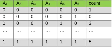
For example, we have a d-dimensional dataset 𝐷
(suppose d is 6):
Table 1. Original dataset
A1 A2 A3 A4 A5 A6 count
0 0 0 0 0 0 1
0 0 0 0 0 1 0
0 0 0 0 1 0 3
… … … …
1 1 1 1 1 1 5
As you can see, the dataset 𝐷 is a table made up of records set as shown in Table 1, which has a capacity of 2𝑑.
The attributes in dataset 𝐷 can be numeric or non-numeric, and non-numeric attributes can be classified for data statistics. The attribute set is defined as 𝐴 = {𝐴1, 𝐴2, ⋯ 𝐴𝑑},
and the domain of an attribute 𝐴𝑖 is represented by Ω 𝑖
which size is |Ω 𝑖|.
The relationship between high-dimensional data is more complicated, and it cannot directly express the relationship between attributes. For example, two attributes of a person such as education and salary, although there is no absolute directional relationship, there is indeed a correlation. Therefore, we first use the Markov network model in the probabilistic graphical model to model the original dataset and graphically represent the relationship between all the attributes:
Fig.1. Establish Markov network A5
A6 A4
A3 A1
After that, we use the noise mechanism to realize differential privacy protection. There are mainly two methods for differential privacy protection in contingency table release: One is to add noise to each cell in the contingency table. This method can maintain the consistency of the marginal frequency of contingency table, but it will cause the large accumulation noise of marginal frequency. The other is to calculate the marginal frequency firstly, and then release them after adding noise to them. The availability of data by the later method is good, but it will break the consistency of marginal frequency. We adopt the second method. Moreover, in order to reduce the amount of noise, we further cluster the Markov network for the subsequent approximate inference and generate the corresponding marginal distribution P(A1A2A3) ,
P(A1A3A4), P(A3A4A5A6) as Fig 2.
Fig.2. Attributes cluster clique
Then, we add noise to each marginal distribution and generate a noise marginal table. At the same time, taking the problem of consistency into account, we use the method in [18] to deal with the consistency.
Finally, combining with the cluster graph and the noise marginal table, the joint distribution of the dataset is obtained and then synthetic data set formed by sampling is released, as Table 2.
Table 2. The joint distribution of the dataset
A1 A2 A3 A4 A5 A6 Probability
0 0 0 0 0 0 0.067
0 0 0 0 0 1 0.003
0 0 0 0 1 0 0.09
… … … …
1 1 1 1 1 1 0.2
In order to verify that the synthetic dataset is similar to the original dataset and the synthetic dataset is available, we need a measure to evaluate the error. Information entropy (KL distance) in information theory can represents the distance between two probability distributions and measure the difference between the two. Because KL distance is asymmetric, we use the smoothed version JS distance of information entropy to measure the approximation of two datasets.
The method proposed in this paper includes the following four steps and the process of PrivMN is showed in Fig.3:
(i) Represent attributes relationship: use a graphical model to represent the relationship between attributes and establish the Markov model. (ii) Approximate inference: infer approximately on the
model based on the method of cluster graph confidence-propagation and obtain a series of low-dimensional marginal tables.
(iii) Generate noisy marginal: add noise to the low-dimensional marginal table by Laplace mechanism to form noisy marginal table.
(iv) Publishing synthetic dataset: combine the noisy marginal tables and the Markov model to generate a synthetic dataset.
Fig.3. The detail steps of PrivMN
4.2. Represent Attributes Relationship
As mentioned before, we use Markov network to represent the relationship between attributes. Firstly, we need to measure the relationship between attributes, there are many kinds of measures, such as chi-square test, mean-square contingency, Cramer's V coefficient, mutual Information and so on. In this paper, we choose mutual information to measure the correlation between two attributes. One reason is that mutual information is different from other correlation coefficients, that it is not limited to real-valued random variables and can express the degree of similarity generally. The other is not only for its small sensitivity but also for its capability of seizing the linear and non-linear correlations.
Given two attributes 𝐴𝑘 and 𝐴𝑙, the mutual information
I(𝐴𝑘, 𝐴𝑙) is defined as:
I(𝐴𝑘, 𝐴𝑙) = ∑ ∑ 𝑝𝑖𝑗𝑙𝑜𝑔 𝑝𝑖𝑗
𝑝𝑖∙𝑝∙𝑗 |Ω𝑙|
𝑗=1 |Ω𝑘|
𝑖=1 (9)
Where 𝑝𝑖𝑗 is the joint distribution of 𝐴𝑘 and 𝐴𝑙. 𝑝𝑖∙=
∑ 𝑝𝑗 𝑖𝑗 and 𝑝∙𝑗= ∑ 𝑝𝑖 𝑖𝑗 is marginal distribution.
In this paper, we consider that 𝐴𝑘 and 𝐴𝑙 are
independent if I(𝐴𝑘, 𝐴𝑙) ≤ θ𝑘𝑙 for some small threshold
θ𝑘𝑙> 0. We choose Cramer's V coefficient as the threshold
and Cramer's V coefficient is a method to calculate the correlation degree of between attributes in contingency table which attribute is greater than 2x2.
Cramer's V coefficient is calculated as follows:
θ𝑘𝑙 = √
𝒳2
𝑛 min [(|Ω𝑘|−1)(|Ω𝑙|−1)]
(10)
Where n is the size of a sample formed by two attributes, the domain of an attribute 𝐴𝑖 is represented by Ω 𝑖 and its
We present the process of establishing Markov network in Algorithm 1:
Algorithm 1 Establish Markov Network
Input: Dataset D with attributes 𝐀 = {𝑨𝟏, 𝑨𝟐, ⋯ 𝑨𝒅}
Input: Privacy parameter 𝛜𝟏
Output: Markov network 𝓗
1: Initialize 𝓗 = (𝑽, 𝑬) with 𝐕 = {𝑨𝟏, 𝑨𝟐, ⋯ 𝑨𝒅} and 𝐄 =
∅;
2: 𝛈 = 𝐋𝐚𝐩 (𝝐𝟏 𝟏);
3: for each attribute pair (𝑨𝒌, 𝑨𝒍) do
4: calculate 𝐈(𝑨𝒌, 𝑨𝒍);
5: if 𝐈(𝑨𝒌, 𝑨𝒍) + 𝜼 ≥ 𝜽𝒌𝒍+ 𝐋𝐚𝐩 ( 𝟏 𝝐𝟏)
then 6: Add edge (𝑨𝒌, 𝑨𝒍) into 𝓗;
7: return 𝓗;
4.3. Approximate Inference
We have obtained the Markov network by Algorithm 1 which reveals attribute relations obviously. Then, we need to infer the model and the purpose of the inference is to achieve the marginal distribution and the conditional distribution of the given model. However, it is still complicated to obtain the required marginal distribution by inferring directly on the Markov network. Therefore, we need further clustering on the Markov network to reduce the computational complexity.
The cluster graph that we constructed in this step is a data structure, which provides a flowchart of the factor processing. Each node in the cluster graph is a cluster associated with a subset of the variables. The graph also contains undirected edges that connect non-empty intersection sets in the domain. Each edge between a pair of clusters 𝐶𝑖 and 𝐶𝑗 is relevant to a cut set S𝑖,𝑗 that S𝑖,𝑗⊆
𝐶𝑖∩ 𝐶𝑗. In addition, we make use of a simple structure
called Bethe clustering graph, which can transform a general clustering graph into a clustering graph satisfying the confidence- propagation algorithm.
We obtain a series of clusters 𝐶𝑖 and cut sets S𝑖,𝑗 after
clustering Markov network that satisfy the family-preserving of cluster graph: Each factor ∅ ∈ Φ is related to a cluster graph 𝐶𝑖 , expressed as α(𝜙), and satisfy
Scope[𝜙] ⊆ 𝐶𝑖.
After obtaining the clustering graph, we ratiocinate in the clustering graph by the confidence-propagation algorithm in Algorithm 2. Confidence-propagation Algorithm of clustering Graph is an approximate calculation and iterative algorithm based on the undirected graph model. It updates the current probability distribution of the entire clustering graph by exchanging information between the nodes in the clustering graph. Moreover, it can solve probabilistic inference problems of the probabilistic graphical model and spread all information on parallel.
After several iterations, the confidence of all nodes is no longer changed. At this time, the clustering graph reaches the convergence state. Moreover, the marginal distribution of each cluster is the optimal solution. This cluster graph is called a cluster graph calibrated, that is, for each edge
(𝑖 − 𝑗) between connected clusters 𝐶𝑖 and 𝐶𝑗 in the cluster
graph, there is
𝜇𝑖,𝑗(S𝑖,𝑗) = ∑𝐶𝑖−S𝑖,𝑗𝛽𝑖(𝐶𝑖)= ∑𝐶𝑗−S𝑖,𝑗𝛽𝑗(𝐶𝑗) (11)
Therefore, the confidence set 𝒬 = {𝛽𝑖:𝑖 𝜖 𝑣𝑒𝑟𝑡𝑒𝑥 𝑠𝑒𝑡} ∪ {𝜇𝑖,𝑗:𝑖 − 𝑗 𝜖 𝑒𝑑𝑔𝑒 𝑠𝑒𝑡} is a
distribution similar to datasets. Where 𝛽𝑖 denotes the
confidence on 𝐶𝑖 and 𝜇𝑖,𝑗 represents the confidence on S𝑖,𝑗.
We present the process of approximate inference in Algorithm 2:
Algorithm 2 Approximate Inference
Input: Markov network 𝓗 Input: Factor set 𝚽 Output: Confidence set 𝓠
1: Bethe cluster graph 𝓤 ←Bethe Graph Create Algorithm (𝓗);
2: confidence set 𝓠← CGraph-SP-Calibrate(𝓤,𝚽); 3: return 𝓠;
4.4. Generate Noisy Marginal
In this section, we use the Laplace mechanism to add noise to the marginal tables of each cluster to generate the noisy marginal tables and consequently realize the differential privacy protection for the attributes in the cluster.
Let the number of clusters be m. For each cluster’s
marginal table, we add Laplace noise Lap (𝑚
𝜖2) to each
entry’s count. Therefore, the privacy budget of a single cluster for privacy protection is 𝜖2
𝑚. According to the
combinatorial property of the differential privacy protection algorithm, the differential privacy protection for different clusters in the same dataset provides the sum of all budgets. Therefore, the noisy marginal tables satisfy 𝜖2
-differential privacy.
In order to reduce the error caused by adding noise and ensure the availability of noise-added data, we will process the noisy marginal tables. We cite the post-processing technique in [22] to ensure consistency even if the noisy marginal tables are of different sizes and attributes are not binary.
Let A = C1∩ C2∩ ⋯ C𝑚≠ ∅, the public attribute of
cluster group. We use 𝑇𝑐𝑖 to denote C𝑖’s noisy marginal
table, 𝑇𝑐𝑖[𝐴] to denote A’s marginal constructed from C𝑖
and 𝑇𝑐𝑖[𝐴] ≡ 𝑇𝑐𝑗[𝐴] to denote that two marginal tables are
identical. We want to ensure 𝑇𝑐1[𝐴] ≡ ⋯ ≡ 𝑇𝑐𝑚[𝐴], that is,
all noisy marginal tables of an attribute are coincident. We achieve this goal in two steps. Where a is a possible value in A’s domain and 𝑇𝐴(𝑎) is the count of a in A’s
noisy marginal table.
(i) Generate the approximate value of 𝑇𝐴(𝑎). The best
estimate of 𝑇𝐴(𝑎) is the minimum noise variance.
Wei Zhang et al.
𝑇𝐴(𝑎) =
∑ 𝑇𝑐𝑖(𝑎)
𝜎𝑖2 𝑚 𝑖=1
∑ 1 𝜎𝑖2 𝑖
(12)
Where 𝜎𝑖2= ∏𝐴𝑗∈(𝑐𝑖\𝐴)|Ω𝑗| is proportional to the
variance of 𝑇𝑐𝑖[𝐴](𝑎).
(ii) Update all 𝑇𝑐𝑖s to be consistent with 𝑇𝐴.
𝑇𝑐𝑖(𝑒) ← 𝑇𝑐𝑖(𝑒) +
𝑇𝐴(𝑎)−𝑇𝑐𝑖(𝑎)
∏𝐴𝑗∈(𝑐𝑖\𝐴)|Ω𝑗| (13)
Where e is the a after the update.
To make all marginal tables consistent, we need to perform a series of mutual consistency steps.
In addition, in order to reduce the bias caused by rounding the negative noisy to 0 and assuring the accuracy, we turn negative counts into 0 while decreasing the counts for its neighbors to maintain overall count unchanged. Specifically, we choose a threshold θ that close to 0. The sum above the threshold is n and the sum below the threshold is k. For each count c above the threshold, we subtract |k| ∗𝑐
𝑛 as the last value of it, and the value below
the threshold becomes 0.
4.5. Publishing Synthetic Datasets
Combining with the previously obtained clustering graph and the noisy marginal tables, we can calculate the joint distribution of attributes. Based on the joint probability calculation formula in Markov networks, the confidence set, and the noisy marginal tables, we can get the non-normalized distribution as follows:
𝒫Φ(ℋ) =
∏ 𝛽𝑖(𝐶𝑖)
∏ 𝜇𝑖,𝑗(S𝑖,𝑗) (14)
The normalization constant is usually obtained by the
sum of all states, that is, Z = ∑𝐶𝑖∏ 𝛽𝑖(𝐶𝑖)
∑S𝑖,𝑗∏ 𝜇𝑖,𝑗(S𝑖,𝑗). Therefore, the
joint distribution is calculated as follows:
𝑃Φ(ℋ) = 1
𝑍𝒫Φ(ℋ) = 1 𝑍
∏ 𝛽𝑖(𝐶𝑖) ∏ 𝜇𝑖,𝑗(S𝑖,𝑗)
(15)
However, directly sampling a synthetic dataset from the joint distribution is computationally prohibitive. Therefore, we use the clustering graph and the noisy marginal tables to generate a synthetic dataset. Specifically, the steps are as follows: 1. Randomly select a cluster in the cluster graph and sample its attributes from its noisy marginal distribution. 2. Continuously sample other attributes in the cliques adjacent to the cliques, that is, they share a common separator, and repeat the above operation. 3. Terminate this process until all the attributes have been sampled.
After the sampling, we calculate the joint distribution by using the joint probability calculation formula given earlier. Thus, we obtain the required joint distribution, which satisfies the differential privacy protection of the complete dataset.
In the four steps of PrivMN, only the first and third steps require access to the original dataset, so we divide the total privacy budget 𝜖 into two portions with 𝜖1 being used for
the first step and 𝜖2 for the third step by the composition
property [8][30]. Therefore, the first and third steps are 𝜖1
-and 𝜖2 -differential privacy respectively, and PrivMN
satisfies 𝜖-differential privacy as a whole, where 𝜖 = 𝜖1+
𝜖2.
5. Evaluation
We make use of three standard real datasets (both binary and non-binary) in our experiments. For binary datasets, we choose Retail referred from [22]. Retail is a retail market basket dataset, where each record consists of the distinct items purchased in a shopping visit. We pre-process Retail to include 50 binary attributes and its domain size is 250. For non-binary datasets, we use the same datasets used in [20]. Adult contains census data from 1994 US census. There are 15 non-binary attributes in it and its domain size is about 252. TPC-E contains
information of ‘Trade’, ‘Security’, ‘Security status’ and ‘Trade type’ tables in the TPC-E benchmark. It consists of 24 non-binary attributes and its domain size is about 277.
We demonstrate the performance of our solution, PrivMN, by comparing with three techniques, namely PrivBayes [20], PriView [15] and JTree[22]. PrivBayes used the directed graph model to reduce the dimensionality of high-dimensional data. PriView used the cover design method in combination principle to select the view and decompose the high-dimensional data into the low-dimensional view, which is a better low-dimensionality reduction method. Therefore, we compare the two algorithms with our method that uses the undirected graph on the performance of dimensionality reduction. Moreover, JTree obtained the low-dimensional marginal table by using the exact inference algorithm named junction in the graph theory after generating a dependency graph. Therefore, we compare the exact inference of this algorithm with the approximate inference algorithm of PrivMN in the experiment.
We evaluate the PrivMN in two aspects: One is the construction of marginal table, which used to measure the accuracy of methods. The other is to train multiple SVM classifiers on the same dataset to predict attributes. We first generate synthetic datasets and then use these datasets to build SVM classifiers. The classification evaluation index mainly includes accuracy, error rate, precision, recall, 𝐹𝑏−
𝑠𝑐𝑜𝑟𝑒, ROC and so on. The correct rate is the most common evaluation index, which is the judgment of all data. The error rate is opposite to the correct rate, which is used to describe the proportion of misclassification by the classifier. The accuracy rate is the measure of accuracy. The recall rate is the measure of coverage rate. The 𝐹𝑏−
𝑠𝑐𝑜𝑟𝑒 is the harmonic average of accuracy and recall, commonly used is 𝐹1. The ROC is a comprehensive index
Since PriView [15] only works for binary datasets and cannot generate synthetic datasets for SVM classification, for binary datasets we only report the results on marginal tables. Due to L2 error and Jensen-Shannon divergence are similar, we use the same evaluation scheme used in PriView, that is, we plot the average L2 error where privacy budget ϵ ∈ {0.1, 1.0} and generate 200 random k-way marginal tables for each k ∈ {4, 6, 8}.
For non-binary datasets, when k is relatively large, a k-way marginal table is normally very sparse and the evaluation scheme used in binary datasets may be significantly biased. Therefore, we choose to follow the same methodology used in PrivBayes [20]. We generate all 2-way and 3-way marginal tables and perform the average total variation distance between the original datasets and the noisy datasets. In addition, we use the same method used in PrivBayes to test the classification results with SVM classifiers. We report the results on Adult, which is the most widely used benchmark dataset for SVM classification analysis. We train SVM classifiers on Adult to predict where an individual (1) is a male, (2) holds a post-secondary degree, (3) has salary > 50k per year, and (4) has never married. We evaluate each classification task with privacy budget ϵ ∈ {0.2, 0.5, 0.8, 1.0}. Each task uses 80% of the datasets as the training set and the remaining 20% for prediction. We employ the misclassification rate as the performance metric.
5.1. Contrast on Binary Datasets
In the first part of experiments, we compare the accuracy of four algorithms on the binary dataset by assigning different privacy budgets. The results are presented in Figure 4.
Fig.4. L2 error of k-way marginal on binary datasets
It can be seen from the figure 4 that our method, PrivMN, is far superior to PrivBayes in most cases and has some advantages over PriView. In Figure 4(a), PriView’s L2 error is higher than PrivBayes when k = 8. It means that PriView is not stable and there is a substantial decrease in the performance of the property with the amount of attributes increase. Although PrivMN is similar to JTree, the error of PrivMN is smaller than JTree. Our method still maintains certain advantages as attributes increase. In general, the advantage of PrivMN is more observable when
ϵ = 0.1, that is, when ε is small, it is still the overall optimal without excessive volatility. Therefore, we consider the synthetic dataset generated by PrivMN can meet different analysis needs. In addition, PrivMN can be applied to non-binary datasets, which is of great significance for practical applications.
5.2. Contrast on Non-Binary Datasets
5.3.1. K-way Marginal Tables
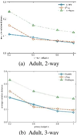
In the second part of the experiment, we compare the average total variation distance of three algorithms for varying privacy budgets on non-binary datasets and present the results in Figure 5.
Since PriView cannot apply to non-binary datasets, we only compare the remaining three methods. It can be seen from the figure that the experimental results of PrivMN are far superior to PrivBayes. Under the condition of different datasets and different k-way marginal tables, the error of JTree is large when ϵ = 0.2, and the overall change range is wide, especially in Figure 5(c)(d). Although PrivMN makes more errors than JTree when ϵ = 0.5 in Figure 5(a)(b), it is relatively flat as a whole. With the gradual increase of the privacy budget, the added noise is less, and the average total variation distance is gradually reducing. Therefore, PrivMN is suitable for extensive datasets and is utility for many real-world applications.
(a) Adult, 2-way
(b) Adult, 3-way (a) Retail, ϵ=0.1
(c) TPC-E, 2-way
(d) TPC-E, 3-way
Fig.5. Total variation distance of k-way marginal tables on non-binary datasets
5.3.2 SVM Classification
In the last part of experiments, we compare the misclassification rate to measure the performance of PrivMN, JTree, and PrivBayes on non-binary datasets. We report the results on Adult with different ϵ values in Figure 6.
Non-Private is the misclassification rate of the original dataset, which is also the best experimental result we can achieve. In figure 6, PrivMN is far superior to privbayes in all cases. Compared with JTree, PrivMN decreases more slowly with different privacy budget, and the overall performance is better. In particular, PrivMN performs even better in Figure 6(a)(b)(c). When ϵ = 0.2 in Figure 6(d), PrivMN has a slight fluctuation, but still within the acceptable range while JTree gets an obvious error. Although the property of the dataset generated by PrivMN is lower than that of the original dataset, it can satisfy the requirement of differential privacy and is superior to general methods. Therefore, PrivMN provides a generic data publishing solutions and it has certain practical significance.
(a) Adult, Y=education
(b) Adult, Y=marital
(c) Adult, Y=gender
(d) Adult, Y=salary
Fig.6. SVM misclassification rates on non-binary datasets
6. Conclusion
Differentially private high-dimensional data publication is one of most challenging research issues and an important problem to be solved urgently. In this paper, we propose to use the Markov network model to represent the mutual relationships between attributes to solve the problem that the direction of relationship between variables cannot be determined in practical application. Moreover, we take advantage of approximate inference to calculate the joint distribution of high-dimensional data under differential privacy to figure out the computational and spatial complexity of accurate reasoning. Experiments on several real standard datasets demonstrate that PrivMN is significant in practice.
Acknowledgments
The authors would like to express their thanks to the anonymous reviewers for their constructive comments and suggestions.
References
[1] The Economist. 2017. The world’s most valuable resource is no longer oil, but data. (May 2017)
[2] Yu S. Big Privacy: Challenges and Opportunities of Privacy Study in the Age of Big Data[J]. IEEE Access, 2017, 4:2751-2763.
[3] Sweeney L. k-anonymity: A model for protecting privacy. International Journal of Uncertainty, Fuzziness and Knowledge-Based Systems, 2002, 10(5): 557-570
[4] Dwork C. Differential privacy//Proceedings of the 33rd International Colloquium on Automata, Languages and programming. Venice, Italy, 2006: 1-12
[5] Koller D, Friedman N. Probabilistic Graphical Models: Principles and Techniques - Adaptive Computation and Machine Learning[M]. MIT Press, 2009.
[6] Roth A, Roughgarden T. Interactive privacy via the median mechanism. Proceedings of the 42nd ACM Symposium on Theory of Computing. Cambridge, USA, 2010: 765-774. [7] Gupta A, Ligett K, McSherry F, et al. Differentially private
approximation algorithms. 2009.
[8] C. Dwork, F. McSherry, K. Nissim, and A. Smith. Calibrating noise to sensitivity in private data analysis. In TCC, 2006.
[9] Hay M, Rastogi V, Miklau G, et al. Boosting the accuracy of differentially private histograms through consistency[J]. Proceedings of the Vldb Endowment, 2010, 3(1-2):1021-1032.
[10] Xiao Y, Gardner J, Xiong L. DPCube: Releasing Differentially Private Data Cubes for Health Information[C]// IEEE, International Conference on Data Engineering. IEEE Computer Society, 2012:1305-1308. [11] Xiao X, Wang G, Gehrke J. Differential Privacy via
Wavelet Transforms. IEEE Transactions on Knowledge and Data Engineering. 2011, 23(8), 1200–1214
[12] Barak B, Chaudhuri K, Dwork C, et al. Privacy, accuracy, and consistency too: A holistic solution to contingency table release//Proceedings of the 26th ACM SIGMOD-SIGACT-SIGART Symposium on Principles of Database Systems, Beijing, China, 2007:273-282
[13] Qardaji W, Yang W, Li N. Differentially private grids for geospatial data[C]// IEEE International Conference on Data Engineering. IEEE Computer Society, 2013:757-768. [14] Rui Chen, Noman Mohammed, Benjamin C. M. Fung, Bipin
C. Desai, Li Xiong: Publishing Set-Valued Data via Differential Privacy. PVLDB 4(11): 1087-1098 (2011) [15] W. Qardaji, W. Yang, and N. Li. Priview: practical
differentially private release of marginal contingency tables. In SIGMOD, 2014.
[16] Xu C, Ren J, Zhang Y, et al. DPPro: Differentially Private High-Dimensional Data Release via Random Projection[J]. IEEE Transactions on Information Forensics & Security, 2017, 12(12):3081-3093.
[17] Ren X, Yu C M, Yu W, et al. LoPub: High-Dimensional Crowdsourced Data Publication with Local Differential Privacy[J]. IEEE Transactions on Information Forensics & Security, 2016, PP(99):1-1.
[18] Pearl J. Probabilistic Reasoning in Intelligent Systems: Networks of Plausble Inference. Morgan Kaufmann Publishers, 1988.
[19] Lauritzen SL, Spiegelhalter DJ. Local computations with probabilities on graphical structures and their application to expert systems. Journal of the Royal Statistical Society. Series B (Methodological), 1988, 50(2):157224.
[20] J. Zhang, G. Cormode, C. M. Procopiuc, D. Srivastava, and X. Xiao. Privbayes: Private data release via bayesian networks. In SIGMOD, 2014.
[21] Su S, Tang P, Cheng X, et al. Differentially private multi-party high-dimensional data publishing[C]// IEEE, International Conference on Data Engineering. IEEE, 2016:205-216.
[22] Chen R, Xiao Q, Zhang Y, et al. Differentially Private High-Dimensional Data Publication via Sampling-Based Inference[C]// ACM SIGKDD International Conference on Knowledge Discovery and Data Mining. ACM, 2015. [23] Hardt M, Rothblum G N. A Multiplicative Weights
Mechanism for Privacy-Preserving Data Analysis[C]// 2010 IEEE 51st Annual Symposium on Foundations of Computer Science. IEEE Computer Society, 2010.
[24] Lee J, Clifton C W. Top-k frequent itemsets via differentially private FP-trees[M]. 2014.
[25] Dwork C. A Firm Foundation for Private Data Analysis[J]. Communications of the Acm, 2011, 54(1):86-95.
[26] Mcsherry F, Talwar K. Mechanism Design via Differential Privacy//Proceedings of the 48th Annual IEEE Symposium on Foundations of Computer Science. Providence, Rhode Island, USA, 2007:94-103.
[27] Hammersley J M, Clifford P. Markov fields on finite graphs and lattices[J]. 1971.
[28] Cliord P. Markov Random Fields in Statistics[J]. Disorder in Physical Systems A, 1990, 14(1):128--135.
[29] Zhang J, Xiao X, Xie X. PrivTree: A Differentially Private Algorithm for Hierarchical Decompositions[C]// International Conference on Management of Data. ACM, 2016:155-170.