http://www.sciencepublishinggroup.com/j/ajmp doi: 10.11648/j.ajmp.20170601.13
ISSN: 2326-8867 (Print); ISSN: 2326-8891 (Online)
New Class of Heintzmann Exact Solution in General
Relativity for an Isotropic Charged Stellar Model
A. H. M. Mahbubur Rahman
1, *, Md. Rubayet Rahman
21Department of Mathematics and Natural Sciences, BRAC University, Dhaka, Bangladesh 2Science and Math Program, Asian University for Women, Chittagong, Bangladesh
Email address:
[email protected] (A. H. M. M. Rahman), [email protected] (Md. R. Rahman)
*Corresponding author
To cite this article:
A. H. M. Mahbubur Rahman, Md. Rubayet Rahman. New Class of Heintzmann Exact Solution in General Relativity for an Isotropic Charged Stellar Model. American Journal of Modern Physics. Vol. 6, No. 1, 2017, pp. 16-22. doi: 10.11648/j.ajmp.20170601.13 Received: January 27, 2017; Accepted: February 13, 2017; Published: March 7, 2017
Abstract:
Exact solution for spherically symmetric isotropic charged fluid sphere are investigated relativistic model of an electrically charged compact star, and energy density associated with the electric fluids is on the same order of magnitude as the energy density of fluid matter itself. The analytic solution depicts a unique static charged configuration of quark matter with radius R~9 km and total mass M~2.5M⊙. And try to inspect the velocity of sound approximately 1/√3 which is similar tothe attitude of SQM (Strange Quark matter). Adiabatic index conform the stability of star if the adiabatic index is less than 4/3. Based on an analytic model in the recent work, the applicable values of physical quantities have been calculated by accepting the estimated masses and radii of some well-known strange star candidates like PSR J1903+327, Her X-1, Cen X-3, EXO 1785-248.
Keywords:
Exact Solution, Einstein – Maxwell, Reissner – Nordström, Relativistic Astrophysics, Compact Star, Equation of State1. Introduction
It is well known that, at the pressure free interface, the Reissner-Nordstrӧm solution is interesting to observe (present charge) the gravitational collapse of a spherical symmetric distribution of the matter to a point singularity may be avoided [1] if the matter distribution acquires large amount of electric charge. Any compact star is not composed of charged perfect fluid and may be used to make a suitable model of compact object with charge matter for the numerical study of the stellar structure [2, 3, 4]. Pant, Metha and Tewari showed that radiative gravitational radiation (GR) collapse may be contributed to formation of the compact non-singular massive hot object [5-7]. The black hole is never formed due to the apparent horizon formation condition [8]. This could be understood as the formation of a naked singularity. But the main reason is that the star radiates all its mass before it reaches the singularity at r = 0 and t = 0. Nuclear matter is meta-stable and it is well known that after releasing a lot of energy converts into strange quark matter (SQM) to achieve stability.
The analytic solutions, behavior of matter, to the equation of relativistic stellar structure of gravitational field equations are two types, one is “normal” matter for neutron stars and
another is “self-bound” strange quark star. Here we study the Self-bound star which is nonlinear electrically charged self-bound stars, self-self-bound star’s radius R< 10-12 km [12]. A self-bound strange quark star belongs to a different class compact object than a conventional normal matter neutron star [12]. For ordinary strange matter, the electric field is ~ 1018 V/cm to up to 1019 V/cm if SQS forms a color
superconductor [9-10]. The electric fields are as high as 10 19-20 V/cm [13] and it’s determined the electrostatic effects and
the surface tension of the interface between vacuum and quark matter [14]. And interesting things is that our model is exactly matching that range [13] of electric field.
known potential strange star candidates to calculate various physical quantities by assuming the estimated masses and predicted radii. And finally Sects. 7 concludes the work.
2. Fundamental Equations
2.1. Field Equations
The interior metric in Schwarzschild coordinates = ( , , , ) [15] is given by the metric:
= ( ) − ( ) − ( + ) (1) The function ( ) and ( ) are arbitrary and satisfy the Einstein-Maxwell field equations,
= − = ( + ) (2) where = 8! is Einstein’s constant. Consequently, and are energy-momentum tensor of fluid distribution and electromagnetic field, assumed in tangential pressure is zero.
For the metric (1), the Einstein–Maxwell field equations with matter and charge expressed as [16].
" #
− #$'%&= ( −) '
* (3)
+ ""− " ", + ,"'+ "# "- # = ( +)'
* (4)
" #
+ #$'%&= . +) '
* (5)
where prime (′) denotes the r-derivative.
For electrically uncharged case, introducing a quantity 0( ) in the following expression
# = 1 − 2( )+)'
' (6)
To transform the system into relatively simpler form eqns. (3)-(5) with the help of following ansatz [18, 19],
= 34(1 + 5 ) (7) Where N is a positive integer and 34, 5 > 0 are two constants to be determined by the appropriate physical boundary conditions. From (3) and (4) one obtain the equation of “pressureisotropy”,
+ ""− " ", + ,"'− "8 "- # + #$%&
' = )
' * (8)
Equation (8) is a second order differential equation in υ and first order in λ. Now we introduce the following
transformations:
# = 9, = 5 (9)
Equation (8) become the following equation by transforming equation (9)
:;
:<+ (( )9 = =( ) (10) This equation is linear differential equation and the solution is
9 = # > ?(<):<@> # > ?(<):<=( ) + A4B (11) Where
(( ) =(C − 2C − 1)) − 2 − 1(1 + )(1 + (1 + C) )
=( ) = (1 + (1 + C) ) E(1 + ) 25F − 1G
and A4 is the integral constant, which may be determined by imposing appropriate physical boundary conditions. Now we can generalize the metric potential Z in general form is
9 = <
( 8<)H%'I 8( 84)<JKLH' >
( 8<)H%KI 8( 84)<JK%HKLH
<' M N) '
< − 1O + A4
<
( 8<)H%'I 8( 84)<JKLH' (12)
2.2. Electric Charge Distribution and Pressure Anisotrop
Various authors presented variety of solutions previously for different suitable choices of charge distributions. Some of the solutions will be found in [23]. In this work we consider the following model distributions:
Model I:
2 2
/ 1 2
2
) 2 1 )( 1 ( ) 4 1 ( 2
x x x
Kx x
Cq
+ + +
= (13)
Model II:
1 2 / 1 2
2
) 1 ( ) 4 1 (
2 =Kx + x +x −
x
Cq (14)
where K ≥ 0.
These distributions are chosen, in term of x, in such a way that
electric field intensity and anisotropy vanish at the center and remains continuous and bounded in the interior of the star for a
wide range of values of the parameters. Thus these choices are physically reasonable and useful in the study of the gravitational behavior of charged stellar objects. It has been shown by Maurya and Gupta [19, 20] for the uncharged and charged cases respectively that the ansatz for the metric function
N
N
x
B
e
υ=
(
1
+
)
where N is a positive integer, produces aninfinite family of analytic solutions of the self-bound type. Some of these were previously known (N = 1, 2, 3, 4, and 5). The most
relevant case is for N = 2, for which the velocity of sound
≈ 1 √3⁄ throughout most of the star, somewhat similar to the behavior of strange quark matter [21]. In this work we keep our interest particularly on to obtain the charged analogue of the types N = 3 which correspond to Heintzmann [22] model and
derive corresponding equations of state.
For the cases N = 3, the solution of the Einstein–Maxwell
Model I: 2 / 1 3 2 / 1 2 3
)
4
1
)(
1
(
)
1
(
2
2
)
4
1
(
)
7
32
40
(
)
1
(
60
x
x
x
A
x
x
x
x
x
x
x
K
e
+
+
+
+
−
+
+
+
+
+
=
−λ (15)
2 / 1 2 3 2 2 / 1 2 3 4
)
4
1
(
)
1
(
7
1
)
1
(
2
)
1
(
9
)
4
1
(
)
7
118
585
1144
760
)(
1
(
60
x
x
x
A
x
x
x
x
x
x
x
x
K
P
C
+
+
+
+
+
−
−
+
+
+
+
+
+
=
κ
(16)2 / 3 2 3 2 2 / 3 2 3 4 5 ) 4 1 ( ) 1 ( ) 3 1 ( 3 ) 1 ( 2 ) 3 ( 3 ) 4 1 ( ) 21 330 2007 5688 7560 3840 )( 1 (
60 x x
x A x x x x x x x x x K
C + +
+ − + + + + + + + + + + − =
ρ
κ
(17)Model II: 2 / 1 3 2 /
1 2(1 ) (1 )(1 4 )
2 ) 4 1 ( ) 1 (
2 x x
x A x x x x x K e + + + + − + + + =
−λ (18)
2 / 1 2 3 2 2 / 1 2
)
4
1
(
)
1
(
7
1
)
1
(
2
)
1
(
9
)
4
1
)(
1
(
)
1
9
11
(
2
x
x
x
A
x
x
x
x
x
x
K
P
C
+
+
+
+
+
−
−
+
+
+
+
=
κ
(19)2 / 3 2 3 2 2 / 3 2 3 ) 4 1 ( ) 1 ( ) 3 1 ( 3 ) 1 ( 2 ) 3 ( 3 ) 4 1 ( ) 1 ( ) 3 17 37 32 (
2 x x
x A x x x x x x x K
C + +
+ − + + + + + + + + − =
ρ
κ
(20)3. Determination of Constants and
Physical Quantities Using Boundary
Conditions
3.1. Conditions for Physical Acceptability
For well behaved nature of the solutions for anisotropic fluid sphere should be satisfied in the following conditions [24]:
i. The solution should be free from physical and geometric singularities i.e. it should yield finite and positive values of the central pressure, central density and nonzero positive value of T(U)= constant, and
# (U)= 1.
ii. The pressure ( and density . should be positive inside the fluid configuration.
iii. The interior solution for strong energy condition should have positive, i.e. (2 ()/. ≥ 0 and dominant energy condition . ≥ (.
iv. The relativistic adiabatic index is given by Γ =
(( + .)( (/ .. the necessary condition for this exact solution to serve ass a model of a relativistic star is that Γ > 4/3.
v. Electric field intensity E, such that (0) = 0, is taken to
be monotonically increasing i.e. ( ⁄ ) > 0 for 0 < < .
vi. Pressure and density, should maximum at the centr and monotoniclly decreasing towards the pressure free interface i.e. ( (/ ) \U= 0, ( ./ ) \U= 0 and ( (/ ) \U< 0, ( ./ ) \U< 0 so that pressure gradient (/ ≤ 0 and density gradient ./ ≤ 0 for 0 < < .
vii. The redshift z should be positive, finite and
monotonically decreasing in nature with the increase of r.
3.2. Determination of the Arbitrary Constant A
To specify A the boundary condition P(r=R)=0can be utilized, Model I:
)
7
1
(
2
)
4
1
)(
9
9
(
)
7
1
(
)
7
118
585
1144
760
(
)
1
(
60
2 / 1 2 3 4 3 3X
X
X
X
X
X
X
X
X
K
A
+
+
−
+
+
+
+
+
+
+
−
=
(21)Model II: ) 7 1 ( 2 ) 4 1 )( 9 9 ( ) 4 1 )( 7 1 ( ) 1 )( 1 9 11 ( 2 2 / 1 2 / 1 2 3 X X X X X X X X K A + + − + + + + + + −
= (22)
Where 2
CR
X
=
3.3. Determination of the Constant B
The constant B can be specified by the boundary condition
e
υ(R)=
e
−λ(R), which yields,2 / 1 4 3 4 2 /
1 2(1 ) (1 ) (1 4 )
2 ) 4 1 ( ) 7 32 40 (
60 x x
x A x x x x x x K B + + + + − + + + + = Model II: 2 / 1 4 3 4 2 / 1
2 2(1 ) (1 ) (1 4 )
2 ) 4 1 ( ) 1 (
2 x x
x A x x x x x K B + + + + − + + + =
3.4. Determination of the Total Charge to Radius Ratio
Model I: 2 / 1 2 2 / 1
2(1 4 ) (1 )(1 2 )
2
+ + +
= K X X X X
R
Q (23)
Model II: 2 / 1 1 2 / 1
2(1 4 ) (1 )
2 + +
= K X X X −
R
Q (24)
3.5. Determination of the Total Mass to Radius Ratio
Model I: 2 / 1 3 2 / 1 2 3 4
)
4
1
)(
1
(
)
1
(
2
3
)
4
1
(
)
7
16
129
488
440
)(
1
(
60
2
X
X
X
A
X
X
X
X
X
X
X
X
X
K
R
M
+
+
−
+
+
+
−
−
+
+
+
=
(25)Model II: 2 / 1 3 2 / 1 2
)
4
1
)(
1
(
)
1
(
2
3
)
4
1
)(
1
(
)
1
3
(
2
2
X
X
X
A
X
X
X
X
X
X
X
K
R
M
+
+
−
+
+
+
+
−
−
=
(26)4. Constructing Physical Realistic Fluid Spheres Pressure and Density Gradients
To analyze the analytical equation of state, a straightforward differentiation of the pressure and density equations (15) – (20) with respect to the auxiliary variable . Due to the comparison of those types we obtain the pressure and density gradients become, Model I: 2 / 3 3 2 3 3 2 / 3 2 3 4 5)
4
1
(
)
1
(
1
14
3
)
1
(
2
)
3
(
9
)
4
1
(
)
37
552
3135
8302
10152
4560
(
20
x
x
x
x
A
x
x
x
x
x
x
x
x
K
dx
dP
C
+
+
−
+
−
+
−
+
+
+
+
+
+
+
=
κ
2 / 5 3 2 3 3 2 /5
(
1
)
(
1
4
)
5
23
30
3
)
1
(
)
5
(
2
3
)
4
1
(
)
(
20
x
x
x
x
A
x
x
x
x
Q
K
dx
d
C
n+
+
+
+
+
+
+
−
+
−
=
ρ
κ
Model II: 2 / 3 3 2 3 3 2 / 3 2 2 3)
4
1
(
)
1
(
1
14
3
)
1
(
2
)
3
(
9
)
4
1
(
)
1
(
)
6
34
59
22
(
2
x
x
x
x
A
x
x
x
x
x
x
x
K
dx
dP
C
+
+
−
+
−
+
−
+
+
+
+
+
+
=
κ
2 / 5 3 2 3 3 2 / 5 2 2 3 4)
4
1
(
)
1
(
5
23
30
3
)
1
(
)
5
(
2
3
)
4
1
(
)
1
(
)
4
10
105
182
64
(
2
x
x
x
x
A
x
x
x
x
x
x
x
x
K
dx
d
C
+
+
+
+
+
+
+
−
+
+
−
+
+
+
−
=
ρ
κ
5. Physical Analysis of the Models
Fig. 1. Adiabatic sound speed for (3.0, 0.11).
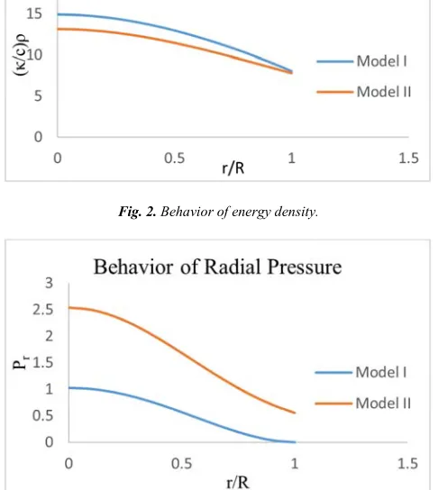
Fig. 2. Behavior of energy density.
Fig. 3. Behavior of radial pressure.
For the particular set of values of (K, X) for which the fluid
distribution satisfies the following inequalities P (r) > 0,
dP/dr < 0, dρ/dr < 0 and dP/ dρ ≥ 0and the speed of sound
satisfies 0 ] ^ (/ . ] 1 and monotonically decreasing with increasing radius are reported in Table 1. A fluid sphere satisfying these inequalities will be termed as well-behaved.
Though there is no explicit relation in between K and X,
these inputs various charged fluid spheres can be generated. The mass and corresponding radius of compact charged fluid spheres, obtained by specifying one of the following: i) central density or, ii) surface density, is reported in Tables 1. For a particular choice of stellar surface density = 8.4×10¹⁴
g cm-3, the total mass and other physical quantities are
calculated and numerical results have been reported in the Table 1.
Model I:
Considering n = 1 the range of values K = 0.8, X = 0.225
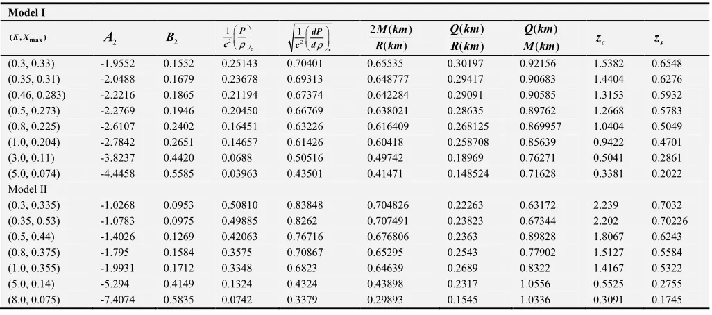
are obtained over which the fluid distribution satisfies the above inequalities. Numerical investigation shows that X decreases as K increases. The maximum values of compactness parameter is obtain (2M/R)max 0.49742, using
Eq. (3.5a) at K= 3.0, Xmax = 0.11. Corresponding to the
values of K and X, the total charge to radius ratio, and total
charge to total mass ratio are Q/R = 0.18969 and Q/M =
0.7671 using Eq. (3.4a). We find out the total mass and other physical quantities are calculated as M = 1.173 M⊙, R = 7.423 Km, ρc =1.41×10¹⁵ gcm-3 and Q =1.294×10²⁰ C for
choosing the stellar surface density ρs = 8.4×10¹⁴ gcm-3 as
parameter. Model II:
For arbitrary value of n = 1 max K=1.0 X= 0.355,
corresponding to these values of K and X the compactness parameter, the speed of sound is 0.6823, total charge to radius ratio and total charge to total mass ratio are found to be (2M/R)max = 0.64639, Q/R = 0.2689 and Q/M = 0.8322. In
order to choosing stellar surface density ρs = 9.2×10¹⁴g cm-3
as parameter the mass and other physical values comes out to be M = 2.15M⊙, R = 9.264 Km, ρc = 2.66×10¹⁵g cm-3. The
maximum mass of charge star depends on the set of lowest values of K and corresponding set of highest values of X. the values of K and X have been plugged in simultaneously as to satisfy dP/dx < 0, dρ/dx < 0 and the speed of sound satisfy 0 ] ^ (/ . ] 1 and monotonically decreasing with increasing radius. It has been observed that the speed of sound always remain less than the speed of light and the condition of causality is satisfied. For large ρ (at center), Γ >
4/3 and there is a minimum value of ρ = ρs the surface value
below which Γ becomes infinitely large.
6. Model for Some Well Known Strange
Star Candidates
estimate of the range of various physical parameters of some potential strange star candidates we have calculated the values of the relevant physical quantities, such as central pressure, and central/surface density, by using the refined mass and predicted radius of 5 pulsars recently reported in Gangopadhyay et al. [27]. The values are reported in Table 2.
7. Conclusion
In this work we have studied particular simple families of relativistic charged stellar models obtained by solving Einstein–Maxwell field equations for a static spherically symmetric distribution of perfect fluid distribution based on two ad hoc assumptions, one for metric potential and other
for the form of electric charge distribution. These families of analytical relativistic stellar models may be considered as charged analogues of Generalized Heintzmann model. Our
analytical analysis shows that, in the presence of charge, the solutions satisfy all the physical requirements to construct
physically acceptable electrically charge stellar models. However, various authors usually have chosen 2×10¹⁴ gcm-3
as stellar surface density to calculate the mass and radius of the charged fluid sphere which may have given rise to the stellar configuration as massive as 4-6 M⊙ with much lower central density. Such massive configuration may not serve as a realistic model for a strange quark star.
For some suitable choices of set of input parameters (K, X),
we have generated compact fluid spheres similar to the mass and radius of some possible strange star candidates like PSR J1614-2230, 4U 1608-52, Vela X-1, Cen X-3.
An analytical stellar model with such physical features is most likely to present an approximated realistic model of strange quark star. And hence the analytical EOS given by our models, besides the usual linear EOS based on phenomenological MIT bag model, could play a significant role in the description of internal structure of electrically charged bare strange quark stars.
Appendix A
Table 1. Model I and II.
Model I
max
(K X, )
2
A B2 2
1 c
P
c ρ 2
1 c
dP c dρ
2 ( )
( )
M km R km
( ) ( )
Q km R km
( ) ( )
Q km
M km zc zs
(0.3, 0.33) -1.9552 0.1552 0.25143 0.70401 0.65535 0.30197 0.92156 1.5382 0.6548
(0.35, 0.31) -2.0488 0.1679 0.23678 0.69313 0.648777 0.29417 0.90683 1.4404 0.6276
(0.46, 0.283) -2.2216 0.1865 0.21194 0.67374 0.642284 0.29091 0.90585 1.3153 0.5932
(0.5, 0.273) -2.2769 0.1946 0.20450 0.66769 0.638021 0.28635 0.89762 1.2668 0.5783
(0.8, 0.225) -2.6107 0.2402 0.16451 0.63226 0.616409 0.268125 0.869957 1.0404 0.5049
(1.0, 0.204) -2.7842 0.2651 0.14657 0.61426 0.60418 0.258708 0.85639 0.9422 0.4701
(3.0, 0.11) -3.8237 0.4420 0.0688 0.50516 0.49742 0.18969 0.76271 0.5041 0.2861
(5.0, 0.074) -4.4458 0.5585 0.03963 0.43501 0.41471 0.148524 0.71628 0.3381 0.2022
Model II
(0.3, 0.335) -1.0268 0.0953 0.50810 0.83848 0.704826 0.22263 0.63172 2.239 0.7032
(0.35, 0.53) -1.0783 0.0975 0.49885 0.8262 0.707491 0.23823 0.67344 2.202 0.70226
(0.5, 0.44) -1.4026 0.1269 0.42063 0.76716 0.676806 0.2363 0.89828 1.8067 0.6243
(0.8, 0.375) -1.795 0.1584 0.3575 0.70867 0.65295 0.2543 0.77902 1.5127 0.5584
(1.0, 0.355) -1.9931 0.1712 0.3348 0.6823 0.64639 0.2689 0.8322 1.4167 0.5322
(5.0, 0.14) -5.294 0.4149 0.1324 0.4324 0.43898 0.2317 1.0556 0.5525 0.2755
(8.0, 0.075) -7.4074 0.5835 0.0742 0.3379 0.29893 0.1545 1.0336 0.3091 0.1745
Appendix B
Table 2. Physical values of energy density and pressure for different strange stars about N=3.
Strange star candidate (k, X) ` (`⨀) R (km) bc,de fc,ge fh,gi
PSR J1614-2230 (0.06, 0.084) 1.38 10.5 0.69 1.618 5.415
(1.5, 0.115) 1.978 11.15 1.19 1.012 6.50
PSR J1903+327 (0.9, 0.16) 1.367 10.495 0.691 0.705 5.525
(1.2, 0.0815) 1.667 10.699 0.655 1.020 6.359
4U 1608-52 (1.17, 0.0816) 1.587 10.452 0.692 0.705 5.522
(6, 0.0866) 1.741 10.751 0.715 0.936 6.501
Vela X-1 (1.17, 0.0817) 1.36 10.421 0.669 0.705 5.524
(6, 0.089) 1.77 10.382 0.711 0.954 6.569
Cen X-3 (3.32, 0.0746) 1.284 10.197 0.621 0.719 5.676
(10, 6, 0.071) 1.49 10.65 0.521 0.9367 6.080
EXO 1785-248 (4.5, 1.4, 0.108) 1.3 10.109 0.547 0.465 6.109
References
[1] Pant, N., Rajasekhara, S.: Variety of well-behaved parametric classes of relativistic charged fluid spheres in general relativity. Astrophys. Space Sci. 333, 161-168 (2011). doi: 10.1007/s10509-011-0607-z.
[2] Nduka, A.: Charged fluid sphere in general relativity, Gen. Relativ. Gravit. 7 (1976) 493―499, doi: 10.1007/BF00766408.
[3] Nduka, A.: Static solutions of Einstein’s field equations for charged spheres of fluid, Acta Phys. Pol. B 9 (1978) 596―571.
[4] Mehra, A. L., Bohra, B. L.: Gen. Relativ. Gravit. 11, 333–336 (1979). doi: 10.1007/BF00759275.
[5] Pant, N., Faruqi, S.: Relativistic modelling of a superdense star containing a charged perfect fluid, Gravit. Cosmol. 18 (2012) 204―210, doi: 10.1134/S0202289312030073. [6] Pant, N., Mehta, R. N., Tewari, B. C., Astrophys. Space Sci.
327, 279 (2010).
[7] Pant, N., Tewari, B. C., Astroph. Space Sci. 331, 645 (2010). [8] Pinheiro, G. and Chan, R., Gen. Rel. Grav. 40, 2149 (2008). [9] Usov, V. V.: Phys. Rev. D, Part. Fields 70, 067301 (2004).
doi: 10.1103/PhysRevD.70.067301.
[10] Usov, V. V., et al.: Astrophys. J. 620, 915 (2005). doi: 10.1086/427074.
[11] Negreiros, R. P., et al.: Phys. Rev. D 82, 103010 (2010). doi: 10.1103/PhysRevD.82.103010.
[12] Farhi, E., Olinto, A., 1986, Astrophys. J. 310, 261.
[13] Negreiros, R. P., et al. Phys. Rev. D 80, 083006 (2009). doi: 10.1103/PhysRevD.80.083006.
[14] Jaikumar, P., Reddy, S., Steiner, A. W.: Phys. Rev. Lett. 96 (2006) 041101.
[15] Tolman, R. C.: Static solutions of Einstein’s field equations for spheres of fluid. Phys. Rev. 55, 364–373 (1939). doi: 10.1103/PhysRev.55.364.
[16] Dionysiou, D. D.: Astrophys. Space Sci. 85, 331 (1982). doi: 10.1007/BF00653455.
[17] Durgapal, M. C.: A class of new exact solutions in general relativity. J. Phys. A, Math. Gen. 15, 2637–2644 (1982). doi: 10.1088/0305-4470/15/8/039.
[18] Lake, K.: All static spherically symmetric perfect-fluid solutions of Einstein’s equations. Phys. Rev. D 67, 104015 (2003). doi: 10.1103/PhysRevD.67.104015.
[19] Maurya, S. K., Gupta, Y. K.: Astrophys. Space Sci. 334, 145 (2011a). doi: 10.1007/s10509-011-0705-y.
[20] Maurya, S. K., Gupta, Y. K.: Astrophys. Space Sci. 334, 301 (2011b). doi: 10.1007/s10509-011-0736-4.
[21] Lattimer, J. M., Prakash, M.: Phys. Rev. Lett. 94, 111101 (2005). doi: 10.1103/PhysRevLett.94.111101.
[22] H. Heintzmann, Z. Physik 228, 489 (1969). doi: 10.1007/BF1558346.
[23] Murad, M. H., Fatema, S.: Int. J. Theor. Phys. 52, 4342 (2013a). doi: 10.1007/s10773-013-1752-7.
[24] Abreu, H. Hernández, L. A Nún᷉ez, Class. Q. Grav. 24, 4631 (2007). doi: 10.1088/0264-9381/24/18/005.
[25] Li, X.-D., et al.: Phys. Rev. Lett. 83, 3776 (1999). doi: 10.1103/PhysRevLett.83.3776.
[26] Dey, M., et al.: Phys. Lett. B 438, 123 (1998). doi: 10.1016/S0370-2693 (98)00935-6.
[27] Weber, F.: Prog. Part. Nucl. Phys. 54, 193 (2005). doi: 10.1016/j.ppnp.2004.07.001.