Analysis and Comparative Study for Developing Computer Network in Terms of Routing Protocols Having IPv6 Network Using Cisco Packet Tracer

(1)

http://www.sciencepublishinggroup.com/j/se doi: 10.11648/j.se.20190702.11

ISSN: 2376-8029 (Print); ISSN: 2376-8037 (Online)

Report

Analysis and Comparative Study for Developing Computer

Network in Terms of Routing Protocols Having IPv6 Network

Using Cisco Packet Tracer

Moshammad Sharmin Akter

*

, Mohammad Anwar Hossain

Department of Information and Communication Engineering, Pabna University of Science and Technology, Pabna, Bangladesh

Email address:

*

Corresponding author

To cite this article:

Moshammad Sharmin Akter, Mohammad Anwar Hossain. Analysis and Comparative Study for Developing Computer Network in Terms of Routing Protocols Having IPv6 Network Using Cisco Packet Tracer. Software Engineering. Vol. 7, No. 2, 2019, pp. 16-29.

doi: 10.11648/j.se.20190702.11

Received: June 13, 2019; Accepted: July 11, 2019; Published: July 23, 2019

Abstract:

Computer technology is growing quickly. Now a day it is the time of internet. Data communication and networking have changed the way we do business and the personal communication. Communication can easily isolate the world through the way of communication. When we communicate, we are sharing information. A routing mechanism needs to add the entire computer system with a higher degree of facility for a network. Routing is the most important part for giving a performance to the network. Network administrators need to performance evaluation based on different criteria for each type of routing protocols. Interior gateway protocols are EIGRP, OSPF, RIP and IS-IS. This paper focuses on the performance of these prominent routers. We chose only three protocols for IPv6 network. These are EIGRPv6, OSPFv3 and RIPng. These protocols are used in IPv6 network in terms of data transfer rate and converge time. These calculate in specific source to destination at simulation environment of cisco. We use ping command in command promote to verify the network connection. It also shows the real time comparison in different perspective. We get the result to use the simulation software cisco packet tracer.

Keywords:

EIGRPv6, OSPFv3, RIPng, Network Model, Simulation, IPv6, Cisco Packet Tracer

1. Introduction

Routing protocol plays the most meaningful importance in

the networking sector. The advantages of data

communication technology provide their services through networking using routing protocols. It transmits packets from source to destination following communication medium. The routing protocols indicate how two routers communicate with each other such as sharing data, resource and information. These routers update their routing table based on previous knowledge to make network adjustable. It also helps routing protocols to select the best path, nodes or routes available on the network. These routing protocol activities are differ from each other. The existence of a router in a network TCP/IP is very important. It takes a routing mechanism that can integrate millions of computers with a higher degree of

flexibility [9]. On the other hand, IPv4 provides addressing space in using 32 bit. 4.3 billion Internet can make through IPv4 protocol addresses [5]. For the fastest growth of internet the IPv4 last address space applicable in February 2012 [10]. Then IPv6 is highly recommended for 2^128 IP addresses with 128 bit addressing space. IPv6 upgrades security mechanism like encryption and evidence using cryptographic key over IPv4 [11].

2. Literature Review

2.1. Related Work

(2)

simulators like cisco packet tracer, OPNET, GNS (Graphical Network Simulator). The researchers tested the different applications based on several parameters and concluded the results. The results showed that EIGRP performance was better in terms of convergence time, CPU utilization, throughput, end-to-end delay, data transfer rate and bandwidth control than RIP and OSPF. In [4], researchers observed and compared the performance of two routing protocols (EIGRPv6 and OSPFv3) with same topologies. In these related works, researchers compared routing protocols with IPv6 network environment because of the necessity in today’s fast growing computer based networks. However, [20, 12] these studies lack the evaluation for the IPv6. Other closely related works are presented in [2, 4, 5, 9] in which authors compared and analyzed two routing protocols (OSPFv3 & EIGRPv6) based on their performance in a small network. In [9], the researchers focused on configuration analysis developing network and compared that IPv6 configuration commands are more complex than IPv4 configuration commands because of IPv6 addresses complexity. Research study [1] showed that OSPF routing protocols provided better QoS (Quality of service) than RIP. In [19] studies, the researchers tested routing protocols in IPv6 network and examined that EIGRPv6 provided more advantage than OSPFv3 in term of Packet transfer in a small network with the help of simulators. These studies did not specifically evaluate the performance of the routing protocols in the hybrid IPv4-IPv6 network. Further very close related works of this paper are [18, 21] in which the researchers compared and analyzed the performance of dissimilar routing protocols in hybrid IPv4-IPv6 network based on different criteria. Besides, the researchers evaluated the performance of routing protocols (EIGRP & OSPF) in IPv4 networks, in pure IPv6 networks and in dual-stack networks based on numerous parameters like (RTT, packet loss, throughput, end-to-end delay, convergence time, jitter, CPU and memory utilization) for user traffic. Also, [7, 20] in these paper, the researchers shows the step by step configuration of OSPF and OSPFv3 routing protocols in IPv4 and IPv6 network using command line interfaces. In these [1-21] papers also contain different comparisons and shows in using figure, data table, comparison table, line graphs, bar charts and so on to represents the research result. It also helps others research followers to relate the work and find out the absolute information and recommendation for future work and research in specific terms.

2.2. IPv6

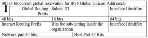
IPv6 address spacing scheme is designed by Internet Engineering Task Force (IETF). IPv6 shows that the address spacing scheme is a 128 bits or 16 bytes, which is represented by a series of eight 16 bits field separated by colons [19]. Now, we show the IPv6 address format as an example is given below:

IPv6 is better for specify to configure addresses in nearly added communication devices to the network. IPv6 is

designed to overcome the IP addresses shortage problems. IPv6 also improves and enhances their services towards compute network over IPv4. IPv6 provides methodology towards multiple IP networks end to end datagram transmission. IPv6 is an internet layer protocol for packet switched internet working.

Figure 1. IPv6 Address Format.

IPv6 feature are given below:

a)Make easy to understand the IP header.

b)It increases scalability and IP addressing capabilities in

routing protocol.

c)It is capable of providing Specifying addresses in near

future and coming IP devices transmission in the internet.

d)It replaces through multicast use on broadcasting the

local link.

e)IPv6 ensures payload encoding, authentication,

encryption for security issues.

f) It provides better real time traffic from end to end

networks example VOIP, Voice and Video than IPv4. So, an IPv6 address is 128 bits or 16 bytes (octets) long, four times the address length in IPv4 [8].

Types of IPv6 addresses are Multicast addresses, Anycast address and Unicast address [7]. Now, Global Unicast IPv6 addresses are given below:

Figure 2. Global Unicast IPv6 Addresses Format.

2.3. Routing Protocols

A routing protocol is a set of rules. It determines the communication mechanism with each other’s. Routing protocols perform several activities, this are-Find out the network, Update and maintain the routing table, Exchange and Communicate for information and data, Decision making and allowing choosing the best route.

There are two type of methods are used for routing protocols, they are:

a)Distance vector (Path vector) protocol: It is known as the

determination of distance vector routing protocol based on distance between the points of origin of the package with the destination point

(3)

protocol for the determination made based on information obtained from other routers [4].

On the other hand, this routing protocol can be divided in two categories:

a)Interior routing protocols: Interior routing protocol is

under a system is called as autonomous system that is used for to allocate the routers between all routers with in internal boundary.

b)Exterior Routing Protocols: Exterior routing protocol is

highly anticipated in autonomous system (AS). An exterior routing protocol is used for external purpose of two multiple routing transmission in autonomous system (AS) or organization.

In network Layer, TCP (transmission control protocol) transmit the information between the routers [19].

2.3.1. RIPng

The routing information protocol next generation (RIPng) is an interior gateway protocol (IGP) that uses a distance vector algorithm that is Bellman-Ford distance-vector algorithm to determine the best route to a destination for data/packet transmission. It uses hop count as the metric. We must be enabling IPv6 to use RIPng. RIPng allows hosts and routers to exchange information for computing routes through an IP-based network. RIPng is a UDP-based protocol and uses UDP port 521. RIPng standards are RFC 2080, RIPng for IPv6. RIPng packets contain command Indicates whether the packet is a request or response message. Request message seek information for the router’s routing table. Response messages sent periodically or when a request message is received. Update messages contain the command and version fields and a set of destinations and metrics. Version number specifies the version of RIPng that the originating router is running. This is currently set to version 1. The rest of the RIPng packet contains a list of routing table entries consisting of the destination prefix (128 bit IPv6 address), Prefix length (number of significant bits in the prefix), Metric (Value of metric advertised for the address), Route tag (The route tag distinguishes external RIPng routes from internal RIPng routes when routes must be redistributed across an EGP (exterior gateway protocol).

2.3.2. OSPFv3

The IPv6 are specified as OSPF version 3 in RFC 5340 (2008). OSPF (Open shortest path first) is a routing protocol comes from network layer for interest protocol (IP) networks. OSPF is a link state routing protocol. It follows the Dijkstra’s algorithm. OSPF determine the best shortest path for the transfer of a packet from source to destination. OSPFv3 is a part of Interior gateway routing protocol (IGP), operating with in a particular organization that is Autonomous System (AS). It is used for large network communication and enterprise transmission. OSPF is used to carry information within a single Autonomous System (AS). It is perform routing calculations based upon data stored with in a Link State Database (LSDB). The OSPF protocol uses area concept. Each area in OSPF is specify with a 32 bit area ID, which are

dotted decimal format and not are compatible with IPv4 addresses, area 0 is the backbone area of an OSPF which is Open Shortest Path First of all OSPF area need to connect to this backbone area which manages all inter area routing [4]. OSPF support VLSM (variable length subnet masking) is used for reduces IP wastage and gives zero percentage wastage [19]. If any changes occurs in the network it updates fast otherwise network is update is slow.

2.3.3. EIGRPv6

The Enhanced Interior Gateway Routing Protocol (EIGRP) is a hybrid routing protocol which provides significant improvements on IGRP [12]. EIGRP replaced IGRP in 1993 since Internet Protocol is designed to support IPv4 addresses that IGRP could not support [13]. Hybrid routing protocol incorporates advantages of both Link-state and Distance Vector routing protocols, it was based on Distance-Vector protocol but contains more features of Link-State protocol [6]. EIGRP (Enhanced Interior Gateway Routing Protocol) is Cisco's proprietary routing protocol based on Diffusing Update Algorithm. EIGRP has the fastest router convergence among the three protocols we are testing [14]. EIGRP saves all routes rather than the best route to ensure the faster convergence. EIGRP keeps neighboring routing tables and it only exchange information that it neighbor would not contain [18]. EIGRP provide a number of tables used to perform routing; the neighbor table stores information about directly associated neighbor routers, the topology table stores loop free paths to destinations as well as route metrics, and successor routes, feasible successors, the final table is the Routing table which provide the lowest cost path for every network [15]. It determine the most efficient (least cost) route to a destination. EIGRPv6 also allow a router to find alternate paths without waiting on updates from other routers. The use of Link Local Addresses to enabled neighbor adjacencies alternately using an IP subnet. EIGRPv6 implements the same evidence mechanism as EIGRP. The formation of a router ID is required to profitably start routing operations. EIGRP is easy to maintain and very fast network convergence with low resource usage and low routing protocol it also supports authentication and has backup routes prepared in the form of successors and feasible successors stored in the topology table, this increases reliability [16]. EIGRP is commonly used in huge networks, and it renew only when a topology changes but not periodically unlike old Distance-Vector protocols which is RIP [17].

2.4. Switch

(4)

3. Network Design Based on Cisco

Packet Tracer

3.1. Network Design Flowchart

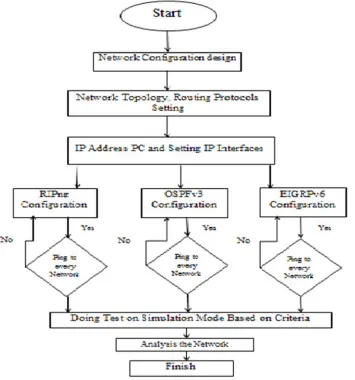
The simulation system design and configuration of the data communication network based on ring topology using RIPng, EIGRPv6 and OSPFv3 routing protocol. Figure 3 showed a flowchart network design. Figure 3 showed the stages in the design and simulation performance of RIPng, EIGRPv6 and

OSPFv3 in a ring topology. This simulation is done on a Cisco Packet Tracer software and configure the network begins with the manufacture of the network topology is a ring topology, setting IP Address, and IP settings on each interface [9]. Each topology configured by the RIPng, EIGRPv6 and OSPFv3 routing protocol then conducted tests ping to every existing PCs after work then proceed to the analysis. It also follows simulation mode for each routing protocols to observe the packet transfer rate based on constant delay and no constant delay criteria.

Figure 3. Network design flowchart for routing protocols.

3.2. Simulation Setup

Packet tracer is a network simulator. Cisco academy creates the Cisco packet tracer. They also provide the free distribution to student and faculty. It is used to configure the routing protocols virtually. It also performs the operations and calculates the time travel for the message from one node to another node [3].

3.3. Network Topology Model

The software used for the simulation is a Cisco Packet

(5)

Figure 4. Packet Tracer environment.

Figure 5. Network topology model.

(6)

Figure 6. Network model which contain three different routing protocols (RIPng, EIGRPv6, OSPFv3) in IPv6 network with simulation environment.

4. Collection of Data from Simulation

Model

The connectivity between different nodes is show by the network. The network consists of different routing protocols that are mainly performed in IPv6 network environment. These protocols are RIPng, OSPFv3, and EIGRPv6. Data collection is carried out using ping command techniques. That is used for check the connectivity from one node to other node in this network. Protocols may be acted different in same network in terms of packet transfer issue from specific source to destination. Figure 6 shows a simulation model of this network for each routing protocols. It helps to calculate and check the time taken for the packet to send and receive to the destination node. We run ping command from the traffic generator to obtain theses data. Then, it runs the simulation using button like Auto/Capture/Play which shows the time. Mainly the time takes by the packet to travel from one station to another station and finally reaching the destination. These data been noted down in tables with their respective station which route the packet takes to reach the destination for three different protocols. Comparisons between three routing protocols with respect to time zone are show in different graphical representation. That is eventually help to find out the decision based on collection of data and corresponding graphical representation of data.

Table 1. Total time taken to travel from node PC0 to PC6 while having RIPng as routing protocol and ICMPv6 as a reference message with no constant delay.

Time in (Second) Last Device At Device Type

0.000 - PC0 ICMPv6

0.003 Switch0 Router0 ICMPv6

0.007 Router0 Router1 ICMPv6

0.008 Router1 Switch2 ICMPv6

0.010 Switch2 PC6 ICMPv6

0.013 PC6 Switch2 ICMPv6

However, the above Table 1 summarizes all connecting nodes that use to pass the data packet from sender to receiver because it doesn’t contain much data. The network is focus on small area concept that’s the reason for the data volume is small. It also shows only one sending and receiving end device as a testing example and their response on specific routing protocol implement on this network with IPv6 environment.

The table above provides information about Total time taken to travel from node PC0 to PC6 while having RIPng as routing protocol. The table contains the data in terms of Time in (second). It shows also the node specific points in terms of Last Device and At Device. The network contains ICMPv6 as a reference message with no constant delay terms. This is IPv6 network environment which having RIPng routing protocol for analyzing the data transfer rate in order of this table with terms of no constant delay.

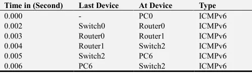
Table 2. Total time taken to travel from node PC0 to PC6 while having RIPng as routing protocol and ICMPv6 as a reference message with constant delay.

0.000 - PC0 ICMPv6

(7)

Now, the above Table 2 summarizes all connecting nodes that use to pass the data packet from sender to receiver because it doesn’t contain much data. The network is focus on small area concept that’s why the data volume is small. It also shows only one sending and receiving end device as a testing example and their response on specific routing protocol implement on this network with IPv6 environment.

The table above provides information about Total time taken to travel from node PC0 to PC6 while having RIPng as routing protocol. The table contains the data in terms of Time in (second). It shows also the node specific points in terms of Last Device and At Device. The network contains ICMPv6 as a reference message with constant delay terms. This IPv6 network environment which having RIPng routing protocol for analyze the data transfer rate in order of this table in terms of with constant delay.

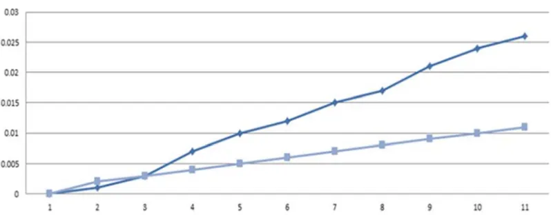
Figure 7. Comparison figure of the RIPng routing protocol in IPv6 with time zone (from Tables 1 and 2) and travels the stations during packet transfer with no constant delay and with constant delay.

The above Figure 7 is a line graph. The line graph illustrates comparison figure of the RIPng routing protocol in IPv6 with time zone. It contains data from Table 1 and 2. The data is collected using RIPng routing protocol in IPv6 network environment using packet transfer with constant delay and with no constant delay terms.

Here, vertical axis of this line graph shows time in (second) and horizontal axis shows total nodes that have been used as a data traveling path. Blue color line graph means RIPng with no constant delay and Red color line graph means RIPng with constant delay.

Now, RIPng shows slightly increased curve at node 1 starting with 0.000 second, then node 2 is 0.003 second and node 3 is 0.007 second for no constant delay term. At that point with constant delay criteria shows data transfer rates for node 1, 2 and 3. These nodes contain time 0.000, 0.002 and 0.003 second. These two curve are also upward trend and slightly straight. Then, RIPng also shows result for node 4, node 5, and node 6. These nodes contain time 0.008, 0.010, and 0.013 second. The curve is upward for increasing data transfer rate with times and nodes. Now, RIPng routing protocol with constant delay term shows the result for nodes

4, 5 and 6 containing time 0.004, 0.005 and 0.006 second. The curve shows the phase of straight upward trend. Now, for node 7 and 8 RIPng gains data transfer rate 0.015 and 0.018 second and the last two nodes these are 9, 10 and RIPng routing protocol gains 0.020 and 0.022 second as data packet transfer rate. The curve shows upward trend. Now, with constant delay criteria for node 7 and 8 RIPng gains data transfer rate 0.007and 0.008 second and the last three nodes these are 9, 10 and RIPng routing protocol gains 0.009, 0.010 second as data packet transfer rate. The curve shows straight upward trend.

(8)

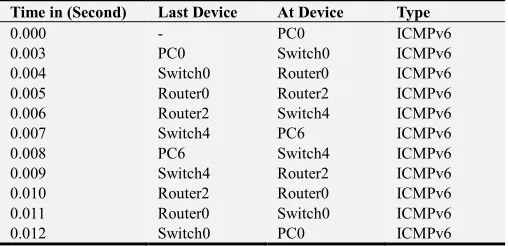
Table 3. Total time taken to travel from node PC0 to PC6 while having OSPFv3 as routing protocol and ICMPv6 as a reference message with no constant delay.

0.000 - PC0 ICMPv6

However, the above Table 3 summarizes all connecting nodes that use to pass the data packet from sender to receiver because it doesn’t contain much data. The network is focus on small area concept that’s why the data volume is small. It also shows only one sending and receiving end device as a testing example and their response on specific routing protocol implement on this network with IPv6 environment.

The table above provides information about Total time taken to travel from node PC0 to PC6 while having OSPFv3 as routing protocol. The table contains the data in terms of Time in (second). It shows also the node specific points in terms of Last Device and At Device. The network contains ICMPv6 as a reference message with no constant delay terms. This IPv6 network environment which having OSPFv3 routing protocol for analyzing the data transfer rate in order of this table with terms of no constant delay. This table also helps to summarize the data about packet transfer rate in specific network model. The data also collects in simulation mode of the Cisco packet tracer software.

Table 4. Total time taken to travel from node PC0 to PC6 while having OSPFv3 as routing protocol and ICMPv6 as a reference message with constant delay.

0.000 - PC0 ICMPv6

Now, the above Table 4 summarizes all connecting nodes that use to pass the data packet from sender to receiver because it doesn’t contain much data. The network is focus on small area concept that’s why the data volume is small. It also shows only one sending and receiving end device as a testing example and their response on specific routing protocol implement on this network with IPv6 environment.

The table above provides information about Total time taken to travel from node PC0 to PC6 while having OSPFv3 as routing protocol. The table contains the data in terms of Time in (second). It shows also the node specific points in terms of Last Device and At Device. The network contains ICMPv6 as a reference message with constant delay terms. This IPv6 network environment which having OSPFv3 routing protocol for analyzing the data transfer rate in order of this table with terms of with constant delay. This table also helps to summarize the data about packet transfer rate in specific network model. The data also collects in simulation mode of the Cisco packet tracer software.

Figure 8. Comparison figure of the OSPFv3 routing protocol in IPv6 with time zone (from Tables 3 and 4) and travels the stations during packet transfer with constant delay and with no constant delay.

The above Figure 8 is a line graph. The line graph illustrates comparison figure of the OSPFv3 routing protocol in IPv6 with time zone. It contains data from Table 3 and 4. The data is collected using OSPFv3 routing protocol in IPv6

network environment using packet transfer with constant delay and with no constant delay terms.

(9)

a data traveling path. Indigo color line graph means OSPFv3 with no constant delay and Blue color line graph means OSPFv3 with constant delay.

Now, OSPFv3 shows slightly increased curve at node 1 starting with 0.000 second, then node 2 is 0.001 second and node 3 is 0.003 second for no constant delay term. At that point with constant delay criteria shows data transfer rates for node 1, 2 and 3. These nodes contain time 0.000, 0.002 and 0.003 second. These two curve are also upward trend and slightly straight with cross section point between them. Then, OSPFv3 also shows result for node 4, node 5, and node 6. These nodes contain time 0.007, 0.010, and 0.012 second. The curve is upward for increasing data transfer rate with times and nodes. Now, OSPFv3 routing protocol with constant delay term shows the result for nodes 4, 5 and 6 gaining time 0.004, 0.005 and 0.006 second. The curve shows the phase of straight upward trend. Now, for node 7 and 8 OSPFv3 gains data transfer rate 0.015 and 0.017 second and the last three nodes these are 9, 10 and 11and OSPFv3 routing protocol gains 0.021, 0.024 and 0.026 second as data packet transfer rate. The curve shows upward trend. Now, with constant delay criteria for node 7 and 8 OSPFv3 gains data transfer rate 0.007and 0.008 second and the last three nodes these are 9, 10 and 11and OSPFv3 routing protocol gains 0.009, 0.010 and 0.011 second as data packet transfer rate. The curve also shows straight upward trend.

The rates of the OSPFv3 with constant delay criteria shows a steady but significant rise of data packet transfer time over the increase of node numbers, while the data packet transfer time with no constant delay experienced a little declined but also significant rise over the increase of node numbers in time. No constant delay line graph also shows little zigzag mode to reach to destination over time and increasing of nodes. In data transfer rate with no constant delay criteria increased sharply throughout the total data traveling path nodes, but with constant delay criteria shows gradual increase in time with the total data traveling path nodes in OSPFv3 routing protocol.

Table 5. Total time taken to travel from node PC0 to PC6 while having EIGRPv6 as routing protocol and ICMPv6 as a reference message with no constant delay.

0.000 - PC0 ICMPv6

However, the above Table 5 summarizes all connecting

nodes that use to pass the data packet from sender to receiver because it doesn’t contain much data. The network is focus on small area concept that’s why the data volume is small. It also shows only one sending and receiving end device as a testing example and their response on specific routing protocol implement on this network with IPv6 environment. That’s result is summarized in the data table. The table above provides information about Total time taken to travel from node PC0 to PC6 while having EIGRPv6 as routing protocol. The table contains the data in terms of Time in (second). It shows also the node specific node points in terms of Last Device and At Device. The network contains ICMPv6 as a reference message with no constant delay terms. This IPv6 network environment which having EIGRPv6 routing protocol for analyzing the data transfer rate in order of this table with terms of no constant delay. This table also helps to summarize the data about packet transfer rate in specific network model. The data also collects in simulation mode of the Cisco packet tracer software.

Table 6. Total time taken to travel from node PC0 to PC6 while having EIGRPv6 as routing protocol and ICMPv6 as a reference message with constant delay.

0.000 - PC0 ICMPv6

(10)

Figure 9. Comparison figure of the EIGRPv6 routing protocol in IPv6 with time zone (from Tables 5 and 6) and travels the stations during packet transfer with constant delay and with no constant delay.

The above Figure 9 is a line graph. The line graph illustrates comparison figure of the EIGRPv6 routing protocol in IPv6 with time zone. It contains data from Table (5, 6). The data is collected using EIGRPv6 routing protocol in IPv6 network environment using packet transfer with constant delay and with no constant delay terms.

Here, vertical axis of this line graph shows time in (second) and horizontal axis shows total nodes that have been used as a data traveling path. In this graph Indigo color line means EIGRPv6 with no constant delay and Blue color line means EIGRPv6 with constant delay.

The rates of the EIGRPv6 with constant delay criteria show a steady but significant rise of data packet transfer time over the increase of node numbers. Now, EIGRPv6 shows slightly increased curve at node 1 starting with 0.000 second, then node 2 is 0.001 second and node 3 is 0.003 second for no constant delay term. At that point with constant delay criteria shows data transfer rates for node 1, 2 and 3. These nodes contain time 0.000, 0.003 and 0.004 second. The curve is also upward trend and slightly straight. Then, EIGRPv6 also shows result for node 4, node 5, and node 6. These nodes contain time 0.006, 0.007, and 0.009 second. The curve is upward for increasing data transfer rate with times and nodes. Now, EIGRPv6 routing protocol with constant

delay term shows the result for nodes 4, 5 and 6 containing time 0.005, 0.006 and 0.007 second. The curve shows the phase of upward trend. Now, for node 7 and 8 EIGRPv6 gains data transfer rate 0.011 and 0.013 second and the last three nodes these are 9, 10 and 11and EIGRPv6 routing protocol gains 0.015, 0.018 and 0.020 second as data packet transfer rate. The curve shows smooth upward trend. Now, for with constant delay criteria node 7 and 8 EIGRPv6 gains data transfer rate 0.008 and 0.009 second and the last three nodes these are 9, 10 and 11and EIGRPv6 routing protocol gains 0.010, 0.011 and 0.012 second as data packet transfer rate. The curve shows high point upward trend. In this curve the data packet transfer time with no constant delay experience a little declined but also significant rises over the increase of node numbers. With no constant delay line graph also shows little cross section mode with constant delay time in early passing the nodes to reach to the destination over time. After increasing of nodes the data transfer rate is also slightly increased to follow these criteria. In data transfer rate with no constant delay criteria increased sharply throughout the total data traveling path nodes, but with constant delay criteria shows gradual but steady increased in time with the total data traveling path nodes in EIGRPv6 routing protocol in IPv6 network environment.

(11)

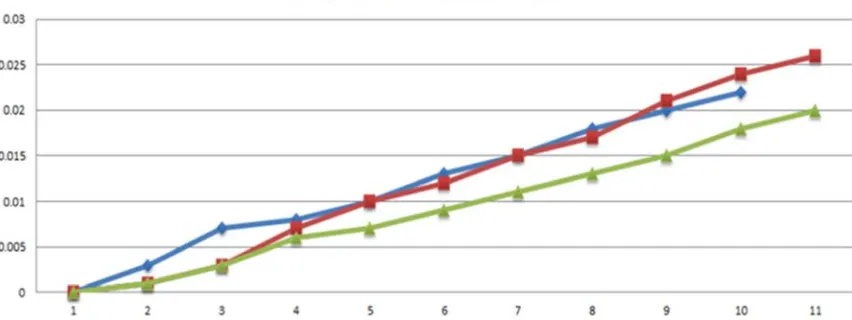
The above Figure 10 is a line graph. It shows the comparison between the routing protocols RIPng, OSPFv3, EIGRPv6 in IPv6 network. It collects the data transfer rate from simulation mode of Cisco packet tracer and tabulate the data in Tables 1, 3, 5 following with no constant delay term.

Here, vertical axis shows Time in (second) and horizontal line shows all path nodes approved by data packet for travelling PC0 sender to PC6 receiver. This is done for the routing protocols. In this line graph green line shows the EIGRPv6 routing protocol data transfer time with no constant delay, red line shows the OSPFv3 routing protocol data transfer time with no constant delay and blue line shows the RIPng routing protocols data transfer time following same criteria.

EIGRPv6 shows slightly increased curve at node 1 it starts with 0.000 second, then node 2 is 0.001 second and node 3 is 0.003 second, compares to same as OSPFv3 routing protocol. But, RIPng is different data rate shows in node 2 and node 3 that is 0.003 second and 0.007 second. Then, EIGRPv6 also shows result for node 4, node 5, and node 6 are 0.006, 0.007, and 0.009 second. The curve is upward for increasing data transfer rate with times and nodes. As the same point OSPFv3 also shows data as 0.007, 0.010, 0.012 second for node 4, 5 and 6. OSPFv3 routing protocol takes more time to

transfer data packets than EIGRPv6 routing protocol. But, RIPng takes 0.008, 0.010, 0.013 second time for node 4, 5 and 6. The line curve is more upward than OSPFv3 and EIGRPv6. For node 7 and 8 EIGRPv6 gains data transfer rate 0.011 and 0.013 second but OSPFv3 gains 0.015 and 0.017 second. So, EIGRPv6 shows downward trend than OSPFv3 above this line graph. But, RIPng gains packet transfer rate 0.015 and 0.018 second for node 7 and 8. At this point RIPng curve is similar to OSPFv3 but little bit upward trend. Now, the last three nodes these are 9, 10 and 11and EIGRPv6 routing protocol gains 0.015, 0.018 and 0.020 second as data packet transfer rate. The curve shows smooth upward trend. On the other hand, OSPFv3 routing protocol gains 0.021, 0.024 and 0.026 second which shows more time taken than EIGRPv6. So, at the end of the point the curve is also more upward trend than EIGRPv6. But, RIPng gains 0.020 and 0.022 second for last two nodes for data transfer rate. The Curve shows little downward for RIPng than OSPFv3 routing protocol. So, OSPFv3 shows as much as straight curve and RIPng shows line graph which is mainly little upward at the beginning then, the curve shows smooth increasing status with time and nodes. This graph helps to find out and eventually make a decision based on the data transfer rate criteria. So the comparison is effectively shown by the Figure 10.

Figure 11. Comparison figure of the RIPng, OSPFv3, EIGRPv6 routing protocol in IPv6 with time zone (from Tables 2, 4, 6) and travels the stations during packet transfer with constant delay.

Above the Figure 11 shows a bar chart. The bar chart provides information about the RIPng, OSPFv3, EIGRPv6 routing protocols in IPv6 with time zone (from Tables 2, 4, 6) and data travels the stations during packet transfer with constant delay criteria. The bar chart summarizes the information by selecting and reporting the main features and makes comparison where relevant. Vertical axis of the bar chart shows the time period of data transfer from source to destination and the horizontal axis shows the total nodes that are used as a data travelling path from sender to receiver.

Here, Blue color bar means EIGRPv6 routing protocol, Indigo color bar means OSPFv3 routing protocol and Violet color bar means RIPng routing protocol.

(12)

node receives data packet at 0.012 second for EIGRPv6 routing protocol.

However, OSPFv3 and RIPng are less than 0.001 second from EIGRPv6. The figure shows a gradually same increase for both these two protocols constant delay for this network. All path nodes are collecting data packet for travelling PC0 sender to PC6 receiver. The last node receives data packet at 0.011 second for OSPFv3 routing protocol. At the same time there is no RIPng routing protocol data transfer rate value because the total nodes are less than OSPFv3 and EIGRPv6 because of the network structure. Data transfer rate for the last node of RIPng routing protocol is 0.011 second.

5. Convergence Time

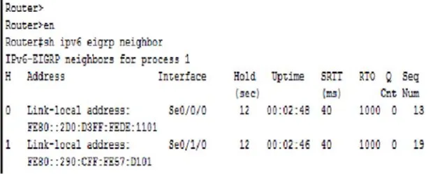
Convergence is also the main design goals. It is also an important performance indicator for routing protocols. Convergence is the state of asset of routers that have the same topological information about the internet work in which they operate. The routing protocols in IPv6 network environment will be examined through the topology [9]. The convergence time for each router to get the information from other routers and ready to transmit data packets through network. Now, EIGRPv6 convergence time is given below:

Figure 12. EIGRPv6 convergence time in IPv6 network.

The convergence time is determined to using CLI command in routers to get the result Column Hold (sec) which indicates the router to wait for the Hello packet from the router to another time. Convergence is every router where the Hello interval by default 5 seconds and Hold/Dead default interval is 15 seconds.

So,

average convergence time 12 12 14 3 12.67

OSPFv3 convergence time is also given below:

Figure 13. OSPFv3 convergence time in IPv6 network.

In OSPFv3, Dead time column where the column shows dead time on the routers to wait for the Hello packets from another router by default Hello interval is 10 seconds and Hold/Dead interval by default 40 seconds.

So,

average convergence time 36 33 31 3 33.33

On the other hand, RIPng has slow time to converge and scalability. In some networking environments [4]. RIPng is not preferred choice for routing over OSPFv3 and EIGRPv6.

6. Data Analysis

To find out the impact of traffic sent and receive in the network eventually meet the result. The simulator was run

(13)

protocols performance. So, the convergence time shows in detail (reference Figure 12 and 13). The average convergence time in this topology shows 12.67 seconds for EIGRPv6 and OSPFv3 routing protocols shows 33.33 seconds.

7. Conclusion

In this paper, the overall analysis is finding performance and advantages in IPv6 network. IPv6 network works based on the routing protocols like RIPng, OSPFv3 and EIGRPv6. This paper helps to analysis time generated by each routing protocols. This traffic generating is done on using ping command in command promote. This evaluation of the routing protocols is working on the simulation mode. It mainly generates different time zone (second) in each station while data packet traveling from one node to other node. The traveling time is different from node to node with no constant delay and constant delay perspective. Plot this generated time zone in a graph to show the comparison and making decision between three different routing protocols. Cisco is used to design an optimal routing topology for developing computer network. So, the data will be collected using simulations and be used to construct accurate performance comparisons of the protocols. EIGRPv6 is comparatively better, faster than RIPng and OSPFv3. If the connections are small of that topology then RIPng become faster. On the other hand, OSPFv3 has advantages in huge networks. It provides hierarchical nature that increases scalability and coverage large areas. OSPFv3 is also applicable for the small and large business organization, enterprises which mainly attempt to connect newly concept of IPv6 network. On the other hand, OSPFv3 converges faster than RIPng. It is better in load balancing. EIGRPv6 convergence time is also very fast. So, EIGRPv6 provides a better performance than RIPng and OSPFv3. EIGRPv6 provides fast convergence time, improved scalability and handling of routing loops. EIGRPv6 has a great impact in ping application. But, in different situation in real life management of networking the routing protocols might be different for adjustment of networking environment.

Acknowledgements

The author would like to thank teachers and classmates from the Data Communication and Networking Research Group of the Department of Information and Communication Engineering of the Pabna University of science and Technology.

References

[1] A. Setiawan and N. Sevani, “Perbandingan Quality Of Service Antara Routing Information Protocol (Rip) Dengan Open Shortest Path First (Ospf),” pp. 196–207.

[2] Gehlot Komal, NC Barwar (2014) Performance Evaluation of EIGRP and OSPF Routing Protocols in Real Time Applications. J. N. V. International Journal of Emerging

Trends & Technology in Computer Science (IJETTCS) 3 (1): 137-143.

[3] Comparison of Routing Protocols in-terms of Packet Transfer Having IPV6 Address Using Packet Tracer, Engineering Technology open access journal, Gajendra Sharma and Binay Sharma Department of Computer Science and Engineering, Kathmandu University, Nepal Submission: September 05, 2018; Published: October 09, 2018 *Corresponding author: Gajendra Sharma, School of Engineering, Kathmandu University, Dhulikhel, Kavre, Nepal.

[4] Comparative Study of EIRGPv6 with OSPFv3 in Internet Routing Protocols, Volume 6, Issue 9, September 2016, ISSN: 2277 128X, International Journal of Advanced Research in Computer Science and Software Engineering Research Paper. Author: Nisha Devi, Er. Brijbhushan Sharma, R. K Saini.

[5] Hinds, A., A. Atojoko, et al. (2013). "Evaluation of OSPF and EIGRP routing protocols for ipv6." International Journal of Future Computer and Communication 2 (4): 287.

[6] Chawda, K. and D. Gorana (2015). A survey of energy efficient routing protocol in MANET. Electronics and Communication Systems (ICECS), 2015 2nd International Conference on, IEEE.

[7] “Study and Optimized Simulation of OSPFv3 Routing Protocol in IPv6 Network” By Md. Anwar Hossain & Mst. Sharmin Akter. Global Journal of Computer Science and Technology: E Network, Web & Security Volume 19 Issue 2 Versions 1.0 Year 2019.

[8] Data Communication and Networking, FIFTH EDITION, written by Behrouz A. Forouzan.

[9] “Developing Computer Network Based on EIGRP Performance Comparison and OSPF”, Lalu Zazuli Azhar Mardedi, Abidarin Rosidi. (IJACSA) International Journal of Advanced Computer Science and Applications, Vol. 6, No. 9, 2015.

[10] McKelvey, F. R. (2013). Internet routing algorithms, transmission and time: toward a concept of transmissive control, York University.

[11] Winter, T. (2012). "RPL: IPv6 routing protocol for low-power and lossy networks."

[12] Islam, M. N. (2010). Simulation based EIGRP over OSPF performance analysis, Blekinge Institute of Technology. [13] Deng, J., S. Wu, et al. (2014). "Comparison of RIP, OSPF and

EIGRP Routing Protocols based on OPNET."

[14] Fiţigău, I. and G. Toderean (2013). Network performance evaluation for RIP, OSPF and EIGRP routing protocols. Electronics, Computers and Artificial Intelligence (ECAI), 2013 International Conference on, IEEE.

[15] Vetriselvan, V., P. R. Patil, et al. (2014). "Survey on the RIP, OSPF, EIGRP Routing Protocols." International Journal of Computer Science and Information Technologies 5 (2): 1058-1065.

(14)

[17] Hoang, T. D. (2015). "Deployment IPv6 over IPv4 network infrastructure."

[18] Wijaya, C. (2011). Performance analysis of dynamic routing protocol EIGRP and OSPF in IPv4 and IPv6 network. Informatics and Computational Intelligence (ICI), 2011 First International Conference on, IEEE.

[19] Comparative Analysis of IS-IS and OSPFV3 with IPV6 Kuldeepika Sharma, Brijbhushan Sharma, R. K. Saini. Volume 6, Issue 9, September 2016, International Journal of Advanced Research in Computer Science and Software Engineering, Research Paper.

[20] Gujarathi Thrivikram, “STUDY AND SIMULATION OF

OSPF ROUTING PROTOCOL USING CISCO PACKET TRACER” (Volume 5, Issue 2, March- April 2016), International Journal of Emerging Trends & Technology in Computer Science (IJETTCS). ISSN 2278-6856.