Performance analysis and optimal power allocation for linear receivers based on superimposed training

R E S E A R C H

Open Access

Performance analysis and optimal power

allocation for linear receivers based on

superimposed training

Abla Kammoun

and Karim Abed-Meraim

Abstract

In this paper, we derive a performance comparison between two training-based schemes for multiple-input multiple-output systems. The two schemes are the time-division multiplexing scheme and the recently proposed data-dependent superimposed pilot scheme. For both schemes, a closed-form expression for the bit error rate (BER) is provided. We also determine, for both schemes, the optimal allocation of power between the pilot and data that minimizes the BER.

Keywords: Superimposed training sequence; MIMO systems performance; Linear receiver

1 Introduction

The use of multiple-input multiple-output (MIMO) antenna systems enables high data rates without any increase in bandwidth or power consumption. However, the good performance of the MIMO systems requires a priori knowledge of the channel at the receiver. In many practical systems, the receiver estimates the chan-nel by time division, multiplexing pilot symbols with the data. Although high quality of the channel estimation could be achieved especially when using a large number of pilot symbols [1], this method may entail a waste of the available channel resources. An alternative method is the conventional superimposed training. It consists in transmitting pilots and data at the same time. However, since during channel estimation, the data symbols act as a source of noise, the channel estimation is affected. In the literature, the impact of channel estimation error upon the performance indexes has been investigated. In [2] and [3], a comparison between the performance of the conventional superimposed training scheme and the time-multiplexing-based scheme has been carried out. The optimal power allocation between pilot and data that maximizes a lower bound of the maximum mutual infor-mation criterion has been provided. It has been shown

*Correspondence: [email protected]

1Alcatel-Lucent, Supélec, Plateau de Moulon, 3 rue Joliot Curie, 91192 Gif-sur-Yvette Cedex, Paris, France

Full list of author information is available at the end of the article

that the use of the optimal conventional superimposed training scheme entails a gain in terms of channel capacity only in special scenarios (many receive antennas and/or short coherence time). In other scenarios, the superim-posed training scheme suffers from high channel estima-tion errors, and its gain over the time-multiplexing-based scheme is often lost. For this reason, many alternatives to the conventional superimposed training scheme have been proposed in recent works.

In [4], Ghogho and Swami proposed to introduce a dis-tortion to the data symbols, prior to adding the known pilot in such a way to guarantee the orthogonality between pilot and data sequences. It is shown that the channel estimation performance is by far enhanced as compared to the standard superimposed scheme. This technique is referred to as the data-dependent superimposed training (DDST). While the DDST scheme exhibits the same chan-nel performance as its time-division multiplexed training (TDMT) counterpart, the effect of the introduced distor-tion may considerably affect the detecdistor-tion performance. The aim of this paper is thus to study the BER perfor-mance of the DDST and TDMT schemes, and to evaluate to which extent the performance of the DDST scheme is altered.

In the literature, the few works focusing on BER per-formance have been based on unrealistic assumptions like the uncorrelation between the noise and channel esti-mation error [5,6]. These assumptions make calculations

feasible for fixed size dimensions but are far away from being realistic. To make derivations possible while keeping realistic conditions, we will relax the assumption of finite size dimensions by allowing the space and time dimen-sions to grow to infinity at the same rate. Working with the asymptotic regime allows us to simplify the derivations, and at the same time, we observe that the obtained results apply as well to usual sample and antenna array sizes. We show also that the obtained expressions can be used to determine the optimal power allocation that minimizes the BER.

The remainder of this paper is as follows: in the next section, we introduce the system model. After that, we review in section 3 the channel estimation and data detection processes for the TDMT and DDST schemes. Section 4 is dedicated to the derivation of the asymptotic BER expressions. Based on these results, we determine the optimal allocation of power between data and training for both schemes. Finally, simulation results are provided in section 7 to validate the analytical derivation.

The following notations are used in this paper: Super-scriptsH, #, and Tr(.) denote Hermitian, pseudo-inverse, and trace operators, respectively. The statistical expecta-tion and the Kronecker product are denoted byEand⊗. The (K ×K) identity matrix is denoted by IK, and the

(Q×Q)matrix of all ones by1Q. The(i,j)th entry of a matrixAis denoted byAi,j.

2 System model and problem setting 2.1 Time-division multiplexing scheme

We consider aM×KMIMO system operating over a flat fading channel. Two phases are considered:

First phase: In the first phase, each transmitting antenna sendsN1pilot symbols. The received symbol

Y1writes as:

Y1=HPt+V1,

wherePtis theK×N1pilot matrix, and

Assumption 1. His the M×K channel matrix with independent and identically distributed (i.i.d.) Gaussian variables with zero mean and variance _K1.

Assumption 2. V1is the M×N1matrix whose

entries are i.i.d. with varianceσ_v2.

Second phase: In the second phase,N2data symbols with powerσ_w2_tare sent by each antenna so that the received signal matrixY2writes as:

Y2=HWt+V2,

where

Assumption 3. Wtis the K×N2data matrix with

i.i.d. bounded data symbols of powerσ_w2_t, andV2is

the M×N2additive Gaussian noise matrix with

entries of zero mean and varianceσ_v2. Moreover,Wt is independent ofV1andV2.

2.2 Data-dependent superimposed training scheme Another alternative to the TDMT-based schemes is to send the training and data sequences at the same time. Since the data is transmitted all the time, these schemes allow efficient bandwidth efficiency but may suffer from the interference caused by the training sequence. Ghogho and Swami [4] proposed thus to distort the data so that is becomes orthogonal to the training sequence. The pro-posed distortion matrixDis defined as:

D=IN−J,

whereJ = K_N1N

K ⊗IK, (we assume that N

K is the integer valued, N being the sample size). This distortion matrix was shown to be optimal in the sense that it minimizes the averaged Euclidean distance between the distorted and non-distorted data [7]. The received signal matrix at each block is therefore given by:

Y=HWd(IN−J)+HPd+V,

where

Assumption 4. Wdis the data matrix with i.i.d. bounded data symbols of powerσ_w2

d, andVis the M×N matrix whose entries are i.i.d. zero mean with varianceσ_v2.

Moreover,Pdis theK×Ntraining matrix. The chosen pilot matrixPdshould fulfill two requirements. It should be orthogonal to the distortion matrix D, thus satisfy-ingDPH

d = 0, and also verify the orthogonality relation

PdPH_d = NσP2dIK in order to minimize the channel esti-mation error subject to a fixed training power. A possible pilot matrix that meets these requirements is

Assumption 5.

Pd(k,n)=σPdexp

j2πkn/K with k=0,· · ·,K−1

and n=0,· · ·,N−1.

(1)

3 Channel estimation and data detection 3.1 TDMT scheme

Ht=Y1PHt

PtPHt

−1

=H+V1PHt

PtPHt

−1

=H+Ht,

where Ht = V1PHt

PtPHt

−1

. Thus, the mean square error (MSE) is written as

MSEt=Mσv2tr

PtPHt

−1

.

As it has been shown in [1], the optimal training matrix that minimizes the MSE under a constant training energy N1σP2tshould satisfy

Assumption 6.

PtPHt =N1σP2tIK,

where σ_P2

t denotes the amount of power devoted to the transmission of a pilot symbol. The optimal minimum value for the MSEtis then given by

MSEt= KMσ_v2

N1σP2t .

In the data transmission phase, the linear receiver uses the channel estimate in order to retrieve the transmitted data. After channel inversion, the estimated data matrix is given by

Wt=Ht

#

Y2,

where Ht

#

denotes the pseudo-inverse matrix of Ht. Assuming that the channel estimation error is small, the pseudo-inverse of the estimated matrix can be approxi-mated by the linear part of the Taylor expansion as [8]:

_Ht#

=H#−H#HtH#+H#

H#HHt

IM−HH#

. (2)

SubstitutingH#byHH_H−1_HH_{in (2), we obtain} Ht

#

=H#−H#HtH#+

HH_H−1_HH

t,

where = IM −HHHH−1HHis the orthogonal pro-jector on the null space of H. Hence, the zero-forcing estimate of the transmitted matrix can be expressed as

Wt=Wt−H#HtWt+

H#−H#HtH#

V2

+HH_H−1_(H

t)HV2.

Consequently, the effective post-processing noiseWt=

Wt−Wtcould be written as

Wt= −H#HtWt+

H#−H#HtH#

+HH_H−1_(H

t)H

V2.

3.2 DDST scheme

The LS channel estimate is obtained by multiplyingYby

PH

d

PdPH_d

−1

, thus giving

Hd=YPHd

PdPHd

−1₌

H+VPH

d

PdPHd

−1₌

H+Hd,

whereHd = VPH_d

PdPH_d

−1

denotes the channel esti-mation error matrix for the DDST scheme. As aforemen-tioned above in Assumption 5, the optimal training matrix that minimizes the MSE should satisfy

PdPHd =NσP2dIK.

The MSE is thus given by:

MSEd=Mσv2tr

PdPHd

−1₌ KMσv2 Nσ_P2

d .

For the DDST scheme, we consider a zero-forcing receiver which, prior to inverting the channel matrix, cancels the contribution of the training symbols by right multiplying

Yby(I−J), where

Y=HWd(IN−J),

the matrixWdbeing the sent data matrix. Thus, the zero-forcing estimate ofWdis given by

Wd=Hd

#

Y(I−J)

=H#−H#HdH#+

HH_H−1_HH

d

×(HWd(I−J)+V(I−J)) =I−H#Hd

Wd(I−J) +H#−H#HdH#

V(I−J)

+HH_H−1_HH

dV(I−J) =Wd(I−J)−H#HdWd(I−J)

+H#−H#HdH#

V(I−J)

+HH_H−1_HH

dV(I−J) =Wd+

−WdJ−H#HdW(I−J) +H#−H#HdH#

V(I−J)

+HH_H−1_HH

Hence,

Wd= −WdJ−H#HdWd(I−J) +H#−H#HdH#

V(I−J)

+HH_H−1_HH

dV(I−J).

4 Bit error rate performance 4.1 TDMT scheme

In order to evaluate the bit error rate performance, we need to evaluate the asymptotic behavior of the post-processing noise observed at each entry of matrixWt. Using the ‘characteristic function’ approach, we can prove that conditioned on the channel matrix, the noise behaves asymptotically like a Gaussian random variable. This result is stated in the following theorem, but its proof is shown in Appendix 1.

Theorem 1. Under Assumptions 1, 2, 3, and 6, and under the asymptotic regime defined as

M,K,N1,N2→ + ∞ with

K N1+N2 →

c1, 0<c1<1

M

K →c2>1 and N2

N1 →

r,

the post-processing noise experienced by the ith antenna at each time k,Wt(i,k), for the TDMT scheme behaves in the asymptotic regime as a Gaussian random variable.

Eej(z∗Wt(i,k))−e−

σ_wt2δt(HHH₎−1

i,i| z|2

4 −−−−−→

K→+∞ 0,

where

δt=c1(1+r)

σ_v2 σ_P2 t

+ σv2

σ2

wt

+c1(1+r)(c2+1)σv4

σ2

wtσ

2

Pt(c2−1) ,

and K→ + ∞refers to this asymptotic regime.

Remark 1. Note that as compared to the results in [9], our results make appear a new additive term of orderσ_v4.

With the Gaussianity of the post-processing noise being verified in the asymptotic case, we can derive the bit error rate for QPSK constellation and Gray encoding as [10]

BER=EQ(√x), (3)

where the expectation is taken with respect to the prob-ability density function of the post processing SNR at the ith branch defined as

γt=

1

δt

(HH_H)−1

i,i .

From [11] and [12], we know that 1

(HHH)−1 i,i

is a weighted

chi-square distributed random variable with 2(M−K+1)

degrees of freedom, whose density function is given by

f(x)= K

M−K+1_xM−K_e−Kx

(M−K)! 1[0,+∞[,

where 1[0,+∞[ is the indicator function corresponding

to the interval [0,+∞[. Hence, the probability density function ofγtis given by

fγt(x)= (Kδt)

M−K+1_xM−K_exp(−Kδ tx)

(M−K)! 1[0,+∞[. (4)

Plugging (4) into (3), we get:

BERt=

(Kδt)M−K+1

(M−K)!

+∞

0

xM−Kexp(−Kδ_tx)Q(√x)dx.

(5)

To compute (5), we use the following integral function:

J(m,a,b)= a

m

(m)

_+∞

0

exp(−ax)xm−1Q(√bx)dx.

(6)

The BER is, therefore, equal to

BER=J(M−K+1,Kδ_t, 1). (7)

The integral in (6) has been shown to have, forc > 0, the following closed-form expression [13]:

J(m,a,b)=

√

c/π (m+1₂)

2(1+c)m+12(m+1)₂

×F1(1,m+

1 2;m+1;

1

1+c), c= b 2a,

where2F1(p,q;n,z)is the Gauss hypergeometric function

[14]. If c = 0 equivalently b = 0, it is easy to note thatJ(m,a, 0)is equal to 1₂. Whenmis restricted to pos-itive integer values, the above equation can be further simplified to [15]

J(m,a,b)= 1

2

1−μ

m−1

k=0

2k k

1−μ2

4

k

, (8)

Plugging (8) into (7), we get

4.2 DDST scheme

Unlike the TDMT scheme, the asymptotic distribution of entries of the post-processing noise matrix is not Gaus-sian. Actually, we prove that

Theorem 2. Under assumptions 4, 5, and under the asymptotic regime defined as

K

N →c1, 0<c1<1 with M

K →c2>1,

the post-processing noise experienced by the ith antenna at each time k behaves asymptotically as a Gaussian mixture random variable, i.e.,

Eexpjz∗[Wd]i,k

andQ is the cardinal of the set of all possible values of

We can also prove that conditioning on the fact that

[W]i,k=1

the post-processing noise satisfies

E

whereQ is the cardinal of the set of all possible values Wi = c1

1

c₁−1

l=1 [W]i,l, and p

i is the probability that Wi takes the valueα_i.

Proof.See Appendix 2.

The assumption of the Gaussianity of the post-processing noise has been always assumed. For time-division multiplexed training, this assumption is well founded, since the post-processing noise converges to a Gaussian distribution in the asymptotic regime (see Theorem 1).

In the superimposed training case, the distortion caused by the presence of data symbols affects the distribution of the post-processing noise which becomes asymptot-ically Gaussian mixture distributed. To assess the sys-tem performance in this particular case, we will start from the elementary definition of the bit error rate. Let

Wi,k denote the post-processing noise experienced at the ith antenna at time k (we omit the subscript d for ease of notations). As it has been previously shown that

Wi,k behaves as a Gaussian mixture random variable. Let σ_d2 be the asymptotic variance of Wi,k, i.e.,σ_d2 =

Using the symmetry of the transmitted data, the BER expression at the ith branch under QPSK constellation and for a given channel realization is given by

BERi=

Hence, conditioned on the channel, the asymptotic bit error rate can be approximated by

BERi,d=

Finally, the proposed approximation of the BER can be obtained by averaging with respect to the channel realizationH, thus giving

BERd=E

For QPSK constellations, it can be shown that#Q =

1

c1, where 1

c1 =

N

K is assumed to be integer. Moreover, the setSof the values taken by(αs)can be given by

σd , then the BER expression becomes

BERd=E

where the expectation is taken over the distribution ofγd given by

fγ_d(x)= (Kδd)

M−K+1_xM−K

(M−K)! exp(−Kδdx).

The computation of the BER can be treated similarly to the TDMT scheme, thus leading to

BERd=

5 Optimal power allocation

So far, we have provided the approximations of the BER for the TDMT and DDST schemes. As it has been pre-viously shown, these expressions depend on the power allocated to data and training, in addition to other param-eters. While the system has no control over the noise power or the number of transmitting and receiving anten-nas, it still can optimize the power allocation in such a way to minimize this performance index. Next, we provide for the TDMT and DDST schemes the optimal data and training power amounts that minimize the BER under the constraint of a constant total power.

5.1 Optimal power allocation for the TDMT scheme Referring to the expressions of BER, we can easily see that the optimal amount of power allocated to data and pilot for the TDMT scheme is the one that min-imizes δt. Let c˜1 = (1 + r)c1, then minimizing δt with respect to σ_w2_t and σ_P2

t under the constraint that N1σ_P2_t+N2σw2t =(N1+N2)σ

2

T (σT2being the mean energy per symbol) results in the following lemma:

5.2 Optimal power allocation for the DDST scheme

For the DDST scheme, we can deduce from (13) that maximizingγdleads to minimize the BER. To maximizeγd, we need to optimizeδdas a function ofσw2dand under the constraint thatσ

2

Pd+(1−c1)σ

2

wd =σ

2

T. After straightforward calculations, we can find that the optimal values forσ_w2

dandσ

2

Pdare given by

Lemma 2. Under the data model, the optimal power allocation minimizing the BER under a total power constraintσ_T2 is given by

σ_w2 d=

(1−c1)

σ_T2+ c1(c2+1)σv2 c2−1

σ_T2

(1−c1)

(1−c1)

σ_T2+ c1(c2+1)σv2 c2−1

+c1σ_T2+ c1(c2+1)(1−c1)σ 2

v c2−1

, (17)

σ_P2 d=

c1σT2+ c1

(c2+1)(1−c1)σv2 c2−1 σ

2

T

(1−c1)

σ_T2+c1(c2+1)σv2 c2−1

+c1σT2+c1

(c2+1)(1−c1)σv2 c2−1

. (18)

6 Discussion

To get more insight into the proposed analysis, we provide here some comments and workouts on the theoretical results derived in the previous sections.

6.1 High SNR behavior of the BER

At high SNRs, the error variance parameters δt andδd are close to zero, and hence, using a first-order Taylor expansion of the BER expressions in (9) and (14), we obtain

BERt≈ 1

2M−K+1(Kδt)

M−K+1

2(M−K)+1 M−K+1

(19)

BERd≈ 1

2c1₁

+O((Kδd)M−K+1), (20)

whereO(x)denotes a real value of the same order of mag-nitude as x. From these approximated expressions, one can observe that the BER at the TDMT scheme is a mono-mial function of the estimation error variance parameter

δ and the number of transmittersK. For example, if the noise power is decreased by a factor 2, then the BER will decrease by 2M−K+1. The diversity gain is thus equal to M− K + 1, which is in accordance with the works in [16] and [5]. Also, we observe that for the DDST case, we have a floor effect on the BER (i.e., the BER is lower bounded by 1

2c1₁) due to the data distortion inherent to this transmission scheme.

6.2 Gaussian vs. Gaussian mixture model

In our derivations, we have found that the post-processing noise in the DDST case behaves asymptotically as a Gaus-sian mixture process, while in most of the existing works, the noise is assumed to be asymptotically Gaussian dis-tributed. In fact, one can show that for large sample sizes (i.e., whenc1 −→ 0), the Gaussian mixture converges to

a Gaussian distribution, allowing us to retrieve the stan-dard Gaussian noise assumption. However, for small or moderate sample sizes, the considered Gaussian mixture model leads to a much better approximation of the BER analytical expression than the one we would obtain with a post-processing Gaussian noise model. In other words, Theorem 2 results allow us to derive closed-form expres-sions for the BER that are valid for relatively small sample sizes.

6.3 Workouts on the optimal power allocation expressions of the TDMT scheme

We consider here two limit cases: (1) The high SNR case, whereσ_v2σ_T2and (2) the case of high-dimensional sys-tem (the number of transmit antennae is of the same order of magnitude as the number of receiver antennae), where c2−1 1. From (16), the data-to-pilot power ratio can

then be approximated by

case (1) σ

2

wt σ_P2 t

≈ _√N1

N2K

(21)

case (2) σ

2

wt σ_P2 t

≈ N1

N2

. (22)

Equation (21) shows that the optimal power allocation in the high SNR case realizes a kind of trade-off between the pilot size and its power, such that the total energy N1σP2tis kept constant. This suggests us to use the smallest possible pilot size that meets the technical constraint of limited transmit power, to increase the effective channel throughput without loss of performance.

(in terms of power allocation) to the channel estimation and to the data detection.

6.4 Workouts on the optimal power allocation expressions of the DDST scheme

A similar workout is considered here for the DDST scheme. We consider the two previous limit cases, and we assume that the sample size is much larger than the num-ber of transmitters, i.e.,NK. In this context, we obtain the following approximations for the data-to-pilot power ratio:

case (1) σ

2

wd σ_P2

d ≈

N

K (23)

case (2) σ

2

wt σ_P2 t

≈1. (24)

Again, we observe that for the large-dimensional system case, one needs to allocate the same total energy to pilot and to the data. For high SNRs, one observes a kind of trade-off between the pilot power and size, but in a differ-ent way than the TDMT case. In fact, if we increase by a factor of 4 the sample size, one can increase the data-to-pilot power ratio by a factor of 2 without affecting the BER performance.

6.5 High SNR BER comparison of the two pilot design schemes

For the DDST scheme, the BER expression can be lower bounded as follows (using the convexity ofQ(√bx) as a function ofb):

BERd= 1

2c1₁−1

1

c₁−1

s=0

1

c1 −1

s

J(M−K+1,Kδ_d, 4s2c2₁)

≥J(M−K+1,Kδ_d, 1 2c1₁−1

1

c₁−1

s=0

1

c1 −1

s

4s2c2₁)

=J(M−K+1,Kδd, 1−c1)

≥J(M−K+1,Kδ_d, 1),

the latter inequality comes from the fact thatJ(m,a,b)is a decreasing function of its last argument. Now, in the high SNR and large sample size scenario (i.e., forσ_v2/σ_T2 1 and N N1,K), we have δt ≈ δd and by continuity J(M−K+1,Kδ_d, 1) ≈ J(M−K +1,Kδ_t, 1) = BERt. Consequently, in this context, the TDMT scheme is better than the DDST in terms of BER, i.e.,

BERd≥BERt.

7 Simulations

Despite being valid only for the asymptotic regime, our results are found to yield a good accuracy even for very small system dimensions. In this section, we present the

simulation results that compare between the TDMT and DDST schemes.

7.1 Performance comparison between DDST- and TDMT-based schemes

In this section, except when mentioning, we consider a 2× 4 MIMO system (K = 2,M = 4) with a data block size N=32.

7.1.1 Bit error rate performance

Figure 1 plots the empirical and theoretical BER under QPSK constellation forN = 32,K = 2, andM = 4 for the TDMT- and DDST-based schemes. All comparisons are conducted in the context when both schemes have the same total energy. The number of training symbols is set toN1=2 (N2=30) for the TDMT scheme.

For low SNR values (SNR below 6 dB), both schemes achieve approximatively the same BER performance, and therefore, the DDST scheme outperforms its TDMT counterpart in terms of data rate, since it has a bet-ter bandwidth efficiency. For high SNR values, the noise caused by the data distortion is higher than the addi-tive Gaussian noise, thus affecting the performance of the DDST scheme.

7.1.2 Applications

To compare the efficiency of the TDMT and DDST schemes, we consider applications in which the BER should be below a certain threshold, say 10−2_{. This may}

be the case for instance of circuit-switched voice applica-tions. Note that for non-coded systems, a target BER of 10−2is commonly used.

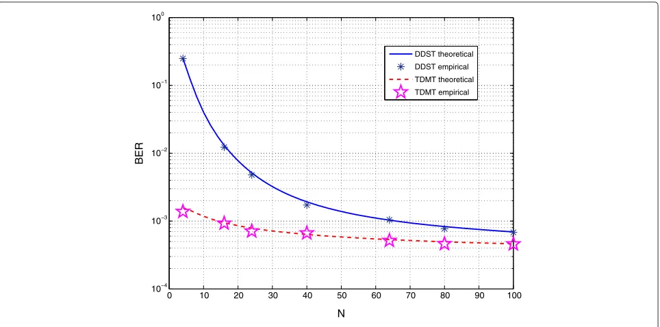
Application 1. In this scenario, we set the SNR σT2 σv2 to 15 dB. We then vary the ratioc1 = _NK from 0.01 to 0.5.

Since we considerK=2 andM=4,N=K/c1varies also

withc1. For each value ofN, we compute the BER using (9)

and (14). Figure 2 illustrates the obtained results. We also superposed in the same plot the empirical results for the TDMT and the DDST scheme. The results show a good match, thereby supporting the usefulness of the derived results.

We note that the DDST scheme may be interesting for long enough frames (N ≥16). For small frames (high dis-tortion ratioc1), the distortion of the data becomes too

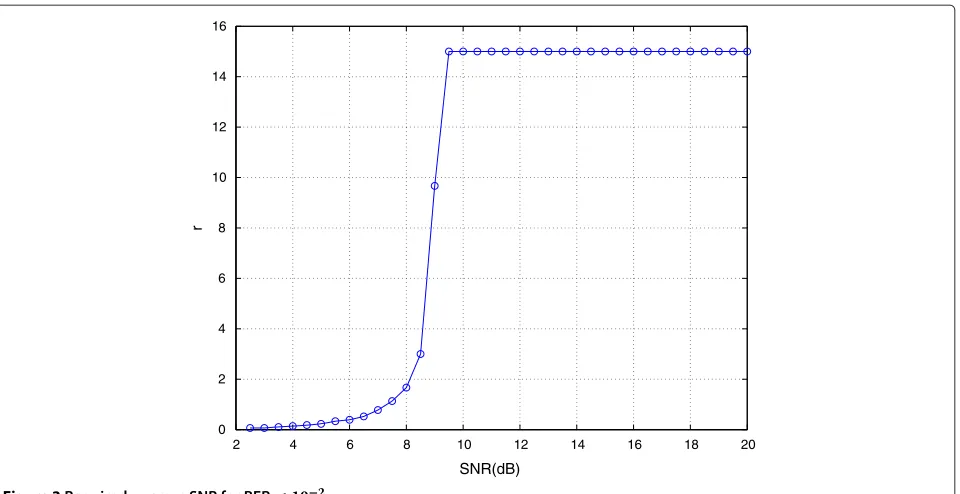
high, thus reducing the interest of the DDST scheme. Application 2. In this experiment, we propose to deter-mine for the TDMT scheme (K = 2,M = 4,N = 32) the optimal ratio N2

N1 that has to be used to meet a certain

quality of service. For that, we consider a scenario where the BER should be below 10−2_{. Using (15), (16), and (9),}

we determine the minimum number of required training symbols to meet the BER lower bound requirement. We, then, plot the corresponding ratior= N2

0 5 10 15 20 25 10−6

10−5 10−4 10−3 10−2 10−1 100

SNR (dB)

BER

DDST empirical BER DDST theoretical BER TDMT empirical BER TDMTtheoretical BER

Figure 1Theoretical and empirical BER for the TDMT- and DDST-based schemes.

the SNR. We note that if the SNR is below 2 dB, the BER requirement could not be achieved. This is to be com-pared with the DDST scheme where the SNR should be set at least to 10.5 dB so as to meet the BER lower bound requirement as it can be shown in Figure 3. Moreover, for a SNR more than 8.5 dB, the minimum number of pilot symbols for channel identification (equal toK) is sufficient to meet the BER requirement.

8 Conclusion

In this paper, we have carried out theoretical studies on BER for two training-based schemes, namely, the basic time-division multiplexed training (TDMT) scheme and the data-dependent superimposed training (DDST)-based scheme. To make derivations possible, the asymptotic regime, where all the system dimensions grow to infin-ity with a constant pace, has been considered. For each

0 10 20 30 40 50 60 70 80 90 100 10−4

10−3 10−2 10−1 100

N

BER

DDST theoretical DDST empirical TDMT theoretical TDMT empirical

2 4 6 8 10 12 14 16 18 20 0

2 4 6 8 10 12 14 16

SNR(dB)

r

Figure 3Requiredrversus SNR for BER≤10−2.

scheme, we have derived closed-form approximations for the BER. We have also determined optimal power alloca-tions of power between data and training that minimize the asymptotic BER.

Appendices Appendix 1 Proof of Theorem 1

In the sequel, we propose to determine the asymptotic dis-tribution of the post-processing noise of each entry of the matrixWt. Actually, the(i,j)entry ofWtis given by

(Wt)i,j= −hi#Htwj+h#i

IK−HtH#

v2,j +,hi(Ht)Hv2,j,

whereh#_i and,hidenote theith row ofH#and

HH_H−1_,

respectively, and wj and v2,j denote the jth columns of

WtandV2, respectively. Conditioned onH,V1, andWt,

(Wt)i,jis a Gaussian random variable with mean equal to−h#_iHtwjand variance

σ_w2_,K =σ_v2h#_i −h#_iHtH#+,hi(Ht)H

×h#_iH−H#HHH

t

h#_iH+Ht

,_hiH_.

Since our proof will be based on the ‘characteristic func-tion’ approach, we shall first recall the expression of the characteristic function for complex random variables:

Theorem 3. Let Xnbe a complex Gaussian random vari-able with mean mX,nand varianceσ_X2_,n, such thatE(Xn− mX,n)2 = 0. Then, Xn can be seen as a two-dimensional

random variable corresponding to its real and imaginary parts. The characteristic function of Xnis, therefore, given by

Eexpj(z∗Xn)

=expjz∗mX,n

×exp

−1 4|z|

2_σ2

X,n

.

Applying Theorem 3, the conditional characteristic function of(W)_i,jcan be written as

Eexpjz∗(Wt)i,j

|V1,H,Wt

=exp−jz∗h#_iHtwj

exp

−1 4|z|

2_σ2

w,K

.

(25)

To remove the condition expectation on V1 and Wt, one should prove thatσ_w2_,K converges almost surely to a deterministic quantity. Actually,σ_w2_,K can be expanded as follows:

σ_w2_,K =σ_v2h#_ih#_iH+σ_v2h#_iHtHHH−1(Ht)h#i

−2σ_v2h_i#Ht(HH)−1h#i

+σ_v2,hiHHtHt

,hi

H

.

Let

Aσ,K =σv2h#iHt

HH_H−1_(H

t)H

h#_iH

Bσ,K =σv2,hiHHtHt

,hi

H

σ,K =h#iHtHHH−1h#i

H

The limiting behavior ofAσ,K can be derived using the following known results describing the asymptotic behav-ior of an important class of quadratic forms:

Lemma 3. [17, Lemma 2.7] Letx = [X1,· · ·,XN]Tbe a N×1vector, where the Xnare centered i.i.d. complex ran-dom variables with unit variance. LetAbe a deterministic N×N complex matrix. Then, for any p≥2, there exists a constant Cpdepending on p only, such that

E----1

Hence, ifAandxhave finite spectral norm and finite eight moment, respectively, we can conclude, using Borel-Cantelli lemma, about the almost convergence of the quadratic form _N1xH_{Ax, thus yielding the following}

corollary:

Corollary 1.Letx=[x1,· · ·,xN]Tbe a N×1vector, where the entries xiare centered i.i.d. complex random variables with unit variance and finite eight order. LetAbe a deter-ministic N × N complex matrix with bounded spectral norm. Then,

1 Nx

H_Ax− 1

NTr(A)−→0 almost surely. By Corollary 1, the asymptotic behavior ofAσ,K is then given by

the dimensions go to infinity [18], we get

Aσ,K −

Note that Theorem 1 can be applied since the smallest eigenvalue of the Wishart matrix(HH)are almost surely uniformly bounded away from zero by(1−√c2)2>0 [19].

Before determining the limiting behavior of Bσ,K, we shall need the following lemma:

Lemma 4. Let Y = √1 Kyi,j

M,K

i=1,j=1 be a M × K with

Gaussian i.i.d entries. Then, in the asymptotic regime given by

Proof.Without loss of generality, we can restrict our proof to the case, wherei= 1. Lety1,· · ·,yK denote the

. Then, using

the formula of the inverse of block matrices, we get

vy= − On the other hand,

Using Corollary 1, we have

yH

the desired result.

We are now in position to deal with the termBσ,K. Using Corollary 1, we get

Using Lemma 4, we get that

i,i converges almost surely to _c1

2−1 (its inverse is the mean of independent

random variables [12]). Then,

Bσ,K− we will be basing on the following result, about the asymptotic behavior of weighted averages:

Theorem 4. Almost sure convergence of weighted aver-ages [20] Leta = [a1,· · ·,aN]Tbe a sequence of N ×1

This theorem was proven in [20] for real variables. Since we are interested in the asymptotic convergence of the real part ofσ,K, it can be possible to transpose our prob-the real parts (respectively, imaginary parts) of aandx. Then,

Referring to Theorem 4, the convergence to zero of σ,K

finite. This is almost surely true, since

1

This leads to

σ_w2_,K− ˜σ_w2_,K −→0 almost surely,

Substituting σ_w2_,K by its asymptotic equivalent in (25), we get

−→0 almost surely.

Also conditioning onWtandH,h#iHtwjis a Gaussian random variable with zero mean and variance

σ_m2_,K = σ

Using the fact that the characteristic function of

h#_iHtwjis

we obtain that conditionally on the channel

Eexpjz∗(Wt)i,j

−→0 almost surely.

We end up the proof by noticing thatσ˜_m2_,K + ˜σ_w2_,K = Proof of Theorem 2

For the DDST scheme, the post-processing noise matrix

Wdis given by respectively, andw˜idenotes theith row of the matrixW.

The vector vT₁,vT₂T is a Gaussian vector. Since

Ev1vH2

=0, we conclude thatv1andv2are independent.

Then,v1andV2 = V

Using the same techniques as before, it can be proved that

and also that h#_iV2H#

h#_iH

−→0 almost surely.

On the other hand, we have

σ_v2(1−c1),hiVH2V2 we get that

σ_v2(1−c1),hiVH2V2 Gaussian random variable with a mean equal tow˜iJjand a varianceσ_w2

Using Corollary 1, we can easily prove that

σ_m2

Conditioning only onH, the conditional characteristic function satisfies:

Giving the structure of the matrixJ,w˜iJj involves the average of _c1

1 symmetric-independent and identically

dis-tributed discrete random variables, and therefore,

Eexp−jz∗w˜i

We conclude the proof by noting that

Competing interests

The authors declare that they have no competing interests.

Acknowledgements

This research has been supported by the ERC Starting Grant 305123 MORE (Advanced Mathematical Tools for Complex Network Engineering).

Author details

1_{Alcatel-Lucent, Supélec, Plateau de Moulon, 3 rue Joliot Curie, 91192}

Gif-sur-Yvette Cedex, Paris, France.2_{PRISME Lab., Ecole Polytechnique de}

l’Université d’Orléans, 12 rue de Blois, BP 6744, 45067, Orléans Cedex 2, France.

Received: 4 January 2013 Accepted: 19 August 2013 Published: 13 September 2013

References

1. B Hassibi, B Hochwald, How much training is needed in multiple-antenna wireless links? IEEE Trans. Inform. Theory49(4), 951–963 (2003) 2. P Bohlin, M Tapio, Performance evaluation of MIMO communication

systems based on superimposed pilots. ICASSP4, 425–428 (2004) 3. M Codray, P Bohlin, Training-based MIMO systems—part I: performance

comparison. IEEE Trans. Signal Process55(11), 5464–5476 (2007) 4. M Ghogho, A Swami,Channel estimation for, MIMO systems using

data-dependent superimposed training. Paper presented at the 42nd Allerton conference on communication and computing, (Monticello, IL, USA, 29 September–1 October 2004)

5. C Wang, EKS Au, RD Murch, WH Mow, RS Cheng, V Lau, On the performance of the MIMO zero-forcing receiver in the presence of channel estimation error. IEEE Trans. Wireless Commun.6(3), 805–810 (2007)

6. EKS Au, C Wang, S Sfar, RD Murch, WH Mow, VKN Lau, RS Cheng, KB Letaief, Error probability for MIMO zero-forcing receiver with adaptive power allocation in the presence of imperfect channel state information. IEEE Trans. Wireless Commun.6(4), 1523–1529 (2007)

7. M Ghogho, A Swami,Optimal training for affine-precoded and

cyclic-prefixed block transmissions. Paper presented at the 2005 IEEE/SP 13th workshop on statistical signal processing, (Novosibirsk, Russia, 17–20 July 2005)

8. JR Magnus, H Neudecker,Matrix Differential Calculus with Applications in Statistics and Econometrics, 3rd edn. (Wiley, Chichester, 2007), p. 450 9. C Wang, EKS Au,Closed-form outage probability and BER of MIMO

zero-forcing receiver in the presence of imperfect CSI. Paper presented at SPAWC ’06 IEEE 7th workshop on signal processing advances in wireless communications, (Cannes, France, 2006), pp. 2–5

10. JG Proakis,Digital Communications, 3rd edn. (McGraw-Hill, New York, 1995)

11. DA Gore, RW Heath, AJ Paulraj, Transmit selection in spatial multiplexing systems. IEEE Commun. Lett.6(11), 491–493 (2002)

12. J Winters, J Salz, R Gitlin, The impact of antenna diversity on the capacity of wireless communication systems. IEEE Trans. Commun.42(234), 1740–1751 (1994)

13. T Eng, L Milstein, Coherent DS-CDMA performance in Nakagami multipath fading. IEEE Trans. Commun.43, 1134–1143 (1995) 14. IS Gradshteyn, IM Ryzhik,Table of Integrals, Series and Products, 7th edn.

(Academic, Amsterdam, 2007), p. 1171

15. R Xu, FCM Lau, Performance analysis for MIMO systems using zero forcing detector over Rice fading channel. Proc. IEEE Int. Symp. Circ. Syst.5, 4955–4958 (2005)

16. A Hedayat, A Nosratinia, Outage and diversity of linear receivers in flat-fading MIMO channels. IEEE Trans. Signal Process.55(12), 5868–5873 (2007)

17. Z Bai, J Silverstein, No eigenvalues outside the support of the limiting spectral distribution of large-dimensional sample covariance matrices. Ann. Probab.26, 316–345 (1998)

18. AM Tulino, S Verdú,Random Matrix Theory and Wireless Communications,. (Now Publishers, New Jersey, 2004), p. 182

19. JW Silverstein, The smallest eigenvalue of a large dimensional Wishart matrix. Ann. Probab.13(4), 1364–1368 (1985)

20. J Baxter, R Jones, M Lin, J Olsen, SLLN for weighted independent identically distributed random variables. J. Theor. Probab.1, 165–181 (2004)

doi:10.1186/1687-1499-2013-227

Cite this article as: Kammoun and Abed-Meraim:Performance analysis and optimal power allocation for linear receivers based on superimposed training.EURASIP Journal on Wireless Communications and Networking2013 2013:227.

Submit your manuscript to a

journal and benefi t from:

7Convenient online submission

7Rigorous peer review

7Immediate publication on acceptance

7Open access: articles freely available online

7High visibility within the fi eld

7Retaining the copyright to your article