An Analytical Approach to Performance Analysis of
Coupled Processor Systems
Christian Vitale
IMDEA Networks, Spain [email protected]
Gianluca Rizzo
HES SO Valais, Switzerland [email protected]
Balaji Rengarajan
Accelera Inc., CA, USA [email protected]
Vincenzo Mancuso
IMDEA Networks, Spain [email protected]
Abstract—We consider a queuing system with coupled pro-cessors (CPS), in which the service rate at each queue varies over time in function of the set of active queues in the system. Performance analysis of CPS has so far been based on simulations or on complex Markov chains under restricting assumptions on input traffic statistics. In contrast, we propose a fully analytical approach to CPS, based on a worst case analysis of system dynamics, and applicable to a large family of traffic character-izations. We derive sufficient conditions for stability for traffic characterized stochastically as well as for traffic constrained by arrival curves, and we show how to compute bounds on backlog and delay. We illustrate our approach and assess our results by means of an example of coupling of wireless transmissions.
I. INTRODUCTION
We consider a system of parallel queues, for which the service rate depends on the set of nonempty queues in the system. Such model, known as Coupled Processors System
(CPS) [1], [2], [3], arises in several contexts, in which coupling derives from resource sharing. In wireless communications, CPS has been proposed to model the complex interdepen-dence among transmitters due to the shared medium and to interference [4]. Given the current trend towards increasing the density of wireless networks, therefore generating more interference, it is becoming essential to take into account in network planning the impact of the interdependency among transmissions. Other applications of the coupled processors model are in clusters of servers, in computing services based on virtualization techniques, and in networks of processors [1], [2], [4]. In such systems, over-provisioning is often the main approach adopted to account for the effects of coupling on performance.
A trivial way of analyzing such systems is to assume a static, worst-case scenario, where service rates are those of a system in saturation, with all queues active. This leads to heavily pessimistic results, often of little practical interest. Re-search has focused therefore on modeling the effects of system dynamics on performance. However, several of these results apply mainly to small, toy scenarios with few queues. The authors of [5], [6] derive closed-form necessary and sufficient conditions for the stability of a CPS composed by just two queues with one class of traffic each, assuming Poisson arrivals and exponential service times. Borst [1] derives a similar result, assuming heavy tailed file size distribution.
For larger settings, some of these approaches require very conservative assumptions, which limit their scope and interest. For a specific inter-cell interference limited cellular networks scenario, Bonald [7] proposes an approximation method which assumes that the demands of all transmitters but one are
smaller than the saturation rate. Results achieved by means of this approximation are typically reliable just when the system approaches saturation, but are loose everywhere else. For CPSs which are already known to be stable, the authors of [3] propose a method for computing bounds on the moments of queue length, based on a semidefinite programming approach. Among the available results, those which apply to more general settings and to a generic number of queues are based on a large number of computationally heavy simulations for their parametrization. The proposals in [8], [2] provide a method to know if a particular configuration of the CPS is stable, based on the steady state probabilities of related Markov chains, and under Poisson traffic assumption. However, the derivation of the steady state probabilities requires a number of simulations which grows factorially with the size of the problem. Fur-thermore, almost all these results assume Poissonian traffic, leaving open the issue of how to derive performance bounds for CPS under different (and possibly more realistic) assumptions on input traffic. In particular, to the best of our knowledge no existing result allows computing deterministic (i.e., hard) sufficient conditions for stability of the system, or of hard bounds on packet delay and backlog.
This paper addresses these issues, and presents a fully ana-lytical approach for performance analysis of a genericN-node CPS, which does not require simulation to be parametrized, and which applies to a large class of input traffic. The main results of our work are:
• We present a general method for the derivation of per-formance bounds in a CPS, based on a (conservative) network model of interactions between queues in a CPS;
• By applying our method to CPSs with independent and stationary sources, as well as to sources constrained by arrival curves, we derive analytical expressions for sufficient conditions for stability of the system, and for bounds on delay and backlog; and
• We illustrate our method on a specific problem in wireless communications, assessing numerically the tightness of our bounds.
Our results suggest that a performance analysis by means of CPS, which models accurately those dynamics induced by coupling, enables a better resource allocation in the considered system.
and we assess them numerically in Section V. Section VI concludes the paper.
II. MODEL ANDASSUMPTIONS
A. System Model
We consider a system of N queues, where each queue receives traffic from one or more fresh sources (i.e., residing out of the system). We assume such queues are served by work conserving schedulers, and that the served traffic leaves the system. The system state at time t is the array ¯a(t), whose i-th element is equal to 0 if thei−th queue is empty, and 1 otherwise. We assume the service rate Ri(t) of queue
i ∈ {1, ..., N} at time t is determined only by the system
state, i.e.,Ri(t) =Ri(¯a(t)). We call such a system aCoupled
Processors System (CPS).
We consider monotonic decreasing CPSs, i.e., if ¯a1 and
¯
a2 are two different states such that ¯a1 ≤ ¯a2,1 then ∀i ∈ {1, ..., N}, Ri(¯a1) ≥ Ri(¯a2). This class of CPSs includes
many problems of practical importance and it has been widely studied in the past, in the context of wireless networks and of bandwidth sharing in packet networks [2]. Without loss of generality, we assume arrivals to be packetized, with a finite number of packet sizes. Finally, we consider that no losses occur in the system at queues (i.e., queues have infinite buffer capacity).
B. Basic Concepts and Definitions
In this section we introduce some definitions and basic results useful for our CPS analysis.
Network Calculus (NC) [9] is a min-plus system theory for deterministic performance analysis of a queuing system. It provides tools for the derivation of bounds to backlog and packet delay in a network. Traffic in NC is typically characterized by means ofarrival curves [9]. LetF represent the set of nonnegative wide-sense increasing functions, and
∀t≥0 letA(t) be the cumulative traffic arrival function for the time interval [0, t]. Thenα∈ F is anarrival curvefor the considered flow if for any[t1, t2],A(t2)−A(t1)≤α(t2−t1).
As such a traffic characterization translates into quite loose assumptions on traffic statistics (mainly involving tail prob-abilities), it applies to a large spectrum of practical settings. One of the most common classes of arrival curves is theleaky bucket arrival curve, whereα(t) =ρt+σ. The non-negative parametersρandσare theleaky bucket rateand theburstiness, respectively.
Let us now introduce the following two notions of stability [9], [10]. Let qi(t)indicate the backlog of queueiat timet.
Definition 2.1 (Stability): A system ofN queues is deter-ministically stable if ∀i∈ [1, ..., N] it exists a Γi <∞ such that
supt≥0qi(t)≤Γi. (1)
The system is stochastically stable if ∀i∈[1, ..., N] it exists aΓi<∞such that
∀t≥0, E[qi(t)]≤Γi. (2)
1Note that for binary vectors¯a
1 and ¯a2, the component-wiseinequality
¯
a1 ≤¯a2 implies that the set of queues active in state¯a1is a subset of the set of queues active in state¯a2.
One can easily see that deterministic stability implies stochas-tic stability, but the converse is not true. Pracstochas-tical sufficient conditions for stability typically imply some constraints on source traffic (e.g., on arrival statistics, or on their arrival curve parameters) and/or on the network (i.e., on some form of service guarantees at queues). For instance, for queues in isolation, a sufficient condition for stochastic (respectively deterministic) stability is that at each queue the average arrival rate be less than the average service rate (respectively, that the leaky bucket rate for the arrivals be less that the minimum service rate) [10].
Definition 2.2 (Continuous Data Scaling Block): For any time interval [t1, t2], with t2 ≥ t1 ≥ 0, let A(t2−t1) be
the amount of bits arrived at a node in the time interval. The node is a continuous data scaling block, with scaling value
S ∈R+, if the amount of bits at its output during the same
time interval is SA(t2−t1).
Scaling blocks have been introduced in Network Calculus in order to model transformation processes which alter the total amount of traffic (lossy channels, data processing, en-coding/decoding, discard of non-conformant traffic).
Definition 2.3 (Policer): A policer with rate Q is a pro-cessing node that, for any arbitrary input traffic, forces Qas the maximum instantaneous departure rate at its output.
In what follows we considerunbufferedpolicers, which discard non-conformant traffic.
Finally, we recall the concept of Generalized Processor Sharing (GPS) node [11]. In general, a GPS node is composed by a server having a fixed service rate R, and M different queues. Each queue is characterized by a weight wi. At any given time, R is split among the non-empty queues proportionally to their weights.
III. ANEW APPROACH TOCPS ANALYSIS
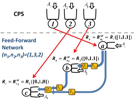
One of the main reasons that accounts for the complexity in studying the performance of CPSs is the fact that correlations between service rates are mutual, which implies circular depen-dencies. To make the problem tractable, we propose a method to break circular dependencies in the analysis. Specifically, we suggest to order the CPS queues and to model the service rate impairment caused by each queue on the queues following in the ordered list, starting from the top of the list (position 1). With this, we model inter-queue dependencies in one direction (top-down in the list). To model the dependencies in the other direction (bottom-up in the list) without incurring in complex calculations, we consider that a queue in position j in the list is considered as always active by all the queues listed in position k < j. This is clearly a worst case approach, which will lead to the identification of performance bounds. Moreover, all possible orderings needs to be considered. In the following we describe the network abstraction that allows to study analytically the performance of a CPS according to the above described methodology (Section III-A) and derive the conditions under which such network abstraction yields performance bounds for a CPS (Section III-B).
A. Feed-forward networks
Fresh Sources
GPS Node
N‐j copies
Sj,1
Sj,j‐1
β1
Scalers Policer
Q
j RateImpairment Fj
βj‐1
βj
βjβj βj
Fig. 1. Structure of thej-th stage of a feed forward network associated to aN-queue CPS.
queues. In such feed-forward networks, dependencies between queues, while still present as in the original CPS, are not mutual. Indeed, the feed-forward structure allows to analyze the network by stages: the activity of a given node, representing a CPS queue, affects only the service rates of those CPS queues which are mapped in following stages of the feed-forward network. Such rate impairment is modeled with an exchange of traffic from the affecting queue to the affected one(s). The effect on queues at preceding stages is modeled instead through a constant penalty on service rates at those stages. This structure allows to apply standard methods for performance analysis, such as classical queuing theory or basic network calculus results.
The structure of the feed-forward networks we propose is the following. Each of such networks has N stages and a two-queue work-conserving GPS node at each stage. GPS nodes are in a one-to one mapping relation with queues of the CPS. Specifically, let j ∈ {1, ..., N} be the label of the
j-th stage of a feed-forward network, as well as of the GPS node in it, and let us label each of the queues of the CPS from 1 toN. Letn¯ = (n1, ..., nj, ..., nN) indicate one of the
N!possible permutations of the labels of the CPS queues. To each permutation n¯ it corresponds a specific mapping which associates the j-th GPS node to thenj-th queue of the CPS.
Fig. 1 describes the general structure of the j-th stage of such feed-forward networks, whereas Fig. 2 shows an example of a three-queue CPS and one of the possible feed-forward networks associated to it. For stage j, each traffic flow βk coming from one of the j−1 previous stages is fed to a dedicated scaling block, with scaling coefficient Sj,k. The aggregate output of all the j−1 scaling blocks is then fed to a policer with rate Qj = (Rupnj −R
sat
nj ), where R
up nj is the
service rate of queue nj of the CPS when the active queues at the CPS are nj, nj+1, ..., nN, andRsatnj when all queues of
the CPS are active.
The output of the policer is finally fed to a dedicated queue of the GPS. The other queue of the GPS is dedicated to traffic from fresh sources. At any time t, we assume arrivals from fresh sources at stage j are the same as at the corresponding queue nj at the CPS. The total capacity of the GPS node is
Rup
nj, which means that the serving rate of the GPS in j-th
stage of the feed-forward network is the minimum possible rate with respect to the state of queues nj+1, ..., nN at the CPS. The GPS weights are w = Rsatnj /R
up
nj for fresh traffic,
and1−wfor traffic from the policer. At the output of the GPS node, traffic coming from stages1, ..., j−1 exits the network. The remaining traffic is fed to a block which producesN−j
exact replicas of the same traffic, introducing no delay. Each
CPS
Feed-Forward Network (n1,n2,n3)=(1,3,2)
1
2
3
a
b
c
Fig. 2. An example of a three-queue CPS, and of a network associated to it, corresponding to the mapping (1,3,2).
replica is fed to one of the following stages.
Let us indicate with Fj(t)the rate impairment at node j. It is the output of the policer at stagej, and models the effect of activity at nodes in stages 1, ..., j−1 on the fresh traffic service rate at node j. Due to the network structure, we have:
Fj(t) = min j−1
X
k=1
βk(¯b(t))Sj,k, Rupnj −R
sat nj
!
. (3)
It is easy to prove that the rate impairment traffic depends only on the activity of theN queues dedicated to fresh traffic.
¯
b(t) is a binary vector which j-th element is zero if at time
t the queue for the fresh traffic at the j-th GPS node of the feed-forward network is empty, one otherwise. The impairment traffic is therefore modeled at the fluid limit as βk(¯b(t)) =
Rupnk−Fk(¯b(t))∀k∈1, ..., j−1.
It is clear that the proposed feed-forward networks are also networks of coupled queues, where coupling translates into rate impairments.
B. Upper Bounding Conditions
In the networks we have described, the scaling coefficients
Sj,k are free parameters. Hence, if S¯ is the matrix of the scaling coefficients of the network, then for a given CPS, each choice of the pair (n¯, S¯) identifies a specific network associated to that CPS. In what follows we present a set of sufficient conditions on rate impairments (and therefore on scaling coefficients) that a feed-forward network must satisfy in order to allow deriving, from its stability, the stability of its associated CPS.
Theorem 3.1: Given a CPS and a (¯n,S¯) feed-forward network associated to it, the stability of this network implies the stability of the CPS (and we say that the network upper bounds the CPS) if the following holds:
Fj(t)≥Rupnj −R 0
nj(t), ∀t≥0∀j ∈ {1, ..., N}; (4)
whereR0nj(t)is the service rate at queuenj of the CPS when the queues of the CPS which are active are all those associated to corresponding active queues in the feed-forward network at
t.
For the proof, please refer to Appendix A.
that at any moment, and at any node of the network, the instantaneous service rate for fresh traffic is always not larger than at the corresponding queue of the CPS. Hence, bounds on backlog and delay for fresh traffic queues in any feed-forward network hold also for the corresponding queue in the CPS.
For a given CPS and a given mapping n¯, Theorem 3.1 identifies a set of feasible arrays S¯, and hence of networks (n¯,S¯). From the structure of the feed-forward network, it can be easily verified that for every mapping ¯n there are at least two choices of scaling coefficients which always satisfy Theorem 3.1.
The first one consists in setting all scaling values to a value larger than the largest possible service rate in the CPS. Note that such a choice is suboptimal, as it is equivalent of studying the system in saturation. A second choice corresponds to setting ∀j∈ {1, ..., N},∀k∈ {1, ..., j−1},
Sj,k=
Rup nj −R
k−up nj
Rupnk
where Rk−up
nj is the service rate at the CPS queue nj when
the CPS queues nk, ..., nN are active. Such values of scaling coefficients make the contribution to interfering traffic from stage kequal to the one we have when stages k, ..., j−1 are active.
IV. SUFFICIENTCONDITIONS FORSTABILITY AND BOUNDS ONBACKLOG ANDDELAY
In the previous section we have seen how to derive a set of upper bounding networks for a given CPS. In what follows we present some sufficient conditions for stability of a CPS, as well as bounds on packet delay and backlog, for two large classes of traffic characterizations, obtained by exploiting the properties of these upper bounding networks.
A. Independent and Stationary Sources
Here we consider the case of a CPS with stationary and independent arrival processes, with average arrival rates
λi (in bits/s), i ∈ {1, ..., N}. For such arrival processes, the following theorem yields sufficient conditions on average arrival rates for the CPS to be stable.
Theorem 4.1: Given anN-queue CPS, with a given set of average arrival rates for its inputs, the CPS is stochastically stable if there exists at least one associated network (¯n,S¯)
satisfying Theorem 3.1 and such that the arrival rates satisfies:
λn1 ≤R
up n1, λnj ≤R
up
nj −E[Fj], ∀j∈ {2, ..., N}, (5)
where:
• E[Fj] is the mean rate impairment at stagej:
E[Fj] =P¯b(j−1)P(¯b(j−1)) min
Pj−1
k=1Sj,kbkβk(¯b(j−1)), Rupnj−Rsatnj
(6)
• ¯b(j−1) is the sub array (b1, ..., bj−1)of the state¯b of the
network. The probability of ¯b(j−1), P(¯b(j−1)), is given
by:
P(¯b(j−1)) =
j−1
Y
k=1
λ
nk
Rnupk−E[Fk]
bk
1− λnk
Rupnk−E[Fk]
1−bk
.
(7)
Proof: see Appendix B. These sufficient conditions are derived by analyzing the upper bounding network by stages, and imposing node stability at each GPS.
It is generally hard to compare our sufficient conditions to existing results, as (except for those assuming saturation in the system) they rely on simulations. For simple 2-queue CPSs, nonetheless, analytic expressions are available [2]. Our conditions for N= 2are:
(
λ1≤Rsat1 ;
λ2≤R2−Rλsat1 1
min(S2,1Rsat1 , R2−R2sat).
(
λ2≤Rsat2 ;
λ1≤R1−Rλsat2
2 min(S2,1R
sat
2 , R1−R1sat).
Such expressions, for the choice of scaling values described
in the previous section (i.e., S2,1=
Rup n2−Rsatn2
Rsat
n1 where{n1, n2}
is{1,2}in the first case and{2,1}in the second) are identical to those derived in [2] and using the theory of deflected random walks [12] or transform methods [13]. Hence for simple cases, our sufficient conditions satisfy the regression test to other approaches, and in particular to [2], whose conditions (valid only for Poisson arrivals) are also necessary. Please note that
Rup n1 =R
sat
n1, since at the first stage all the queues mapped into
the following stages are considered as always active.
When the sufficient conditions in Theorem 4.1 hold, it is possible to derive mean backlog and delay by exploiting standard queuing theory results. For instance, when arrivals are Poisson and packet lengths are exponentially distributed, the fresh arrivals queue at any stage j of the upper bounding network can be modeled as an M/G/1 queue. Its mean backlog E[qj]is therefore given by:
E[qj] =
ρj
1−ρj
E[τ2
j]
2E[τj]
, (8)
where ρj is the mean queue utilization, given by λnj Rupnj−E[Fj],
and τj is the packet processing time for fresh arrivals at the
j-th stage. E[τj] can be computed by exploiting the law of total expectation
E[τj] = X
¯
b(j−1)
E[τj|¯b(j−1)]P(¯b(j−1)).
E[τj|¯b(j−1)] is derived assuming the node has exponential
service times, with mean Rup L
nj−Fj|¯b(j−1).Lis the mean packet
size, while Fj|¯b(j−1) is the mean rate impairment at stage j
when the state of queues1toj−1is given by¯b(j−1), and it can
be derived from Eq. (6). The derivation of E[τj2]follows the same steps. Furthermore, mean packet delay is derived from
E[qj]by using Little’s law.
inner bounds obtained through all the networks satisfying the hypothesis of that theorem. Similarly, the ultimate bounds to backlog and delay can be derived as the min across all such networks.
B. Traffic Constrained by Arrival Curves
In what follows, we assume fresh traffic is constrained by arrival curves. More specifically, we consider leaky bucket arrival curves, despite similar results can be derived through our method for other types of arrival curves. The following theorem defines a set of sufficient conditions on leaky bucket rates for the deterministic stability of the CPS.
Theorem 4.2: Given anN-queue CPS, where at each node
j = 1, ..., N fresh arrivals are constrained by leaky bucket
arrival curves, with parameters (ρj, σj), the CPS is determin-istically stable if there exists at least one associated network
(¯n,S¯) satisfying Theorem 3.1, and such that at each stage
j = 1, ..., N,ρnj satisfies
ρnj ≤max R
sat nj , R
up nj −
j−1
X
k=1
Sj,kρnk
!
. (9)
For the proof see Appendix C. From Eq. (9) we see that a trivial sufficient condition for stability isρj≤Rnsatj ,∀j, which
corresponds to assuming the whole system is in saturation (all queues active). The additional terms in (9) take into account the fact that queues are not always active, and they are function of the bounds to fresh traffic at those nodes which affect the service rate of the considered node.
When a CPS is stable according to Theorem 4.2, the set of upper bounding network(s) can be used to compute hard bounds to delay and backlog for the CPS.
Theorem 4.3: Let us consider a CPS and an (¯n,S¯) upper bounding network which verifies the hypothesis of Theo-rem 4.2. Then a bound for backlog at each node nj of the CPS, j= 1, ..., N is given by:
σn∗j =σnj+
(ρnj −R
sat nj )
+Pj−1 k=1Sj,kσ
∗
nk
Rupnj −R
sat nj −
Pj−1 k=1Sj,kρnk
. (10)
Moreover, if the nodes of the CPS are FIFO, a bound to packet delay at the same node is:
dnj=
σnj Rsat
nj , ifρnj ≤R
sat
nj andσnj ≤cnj,
Tnj +
σnj Rupnj−Pj−1
k=1Sj,kρnk
, ifσnj > cnj,
cnj Rsat
nj
−cnj−σnj
ρnj , ifρnj> R
sat
nj andσnj≤cnj.
(11)
with:
cnj =
∞, ifRsat
nj ≥R
up nj −
Pj−1
k=1Sj,kρnk,
Rsat nj
Pj−1 k=1Sj,kσnk∗
Rupnj−Rsat
nj−
Pj−1
k=1Sj,kρnk otherwise.
Tnj =
Pj−1 k=1Sj,kσ
∗
nk
Rupnj −
Pj−1 k=1Sj,kρnj
.
Please note that cnj is infinite just if ρnj ≤ Rnj (from
Eq. (9)). Therefore, there is no configuration for the arrivals
TX 1
RX 1
TX 2 RX 2
TX 3
RX 3
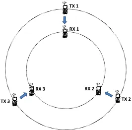
Fig. 3. Scenario under analysis, with three transmitter-receiver pairs.
TABLE I. SETUPSCENARIO
Bandwidth 20M Hz
d 10m
Transmit powerPT X 200 mW Max. packet length 1500B Max. transmission rateCM AX 90M b/s
Path loss exponent 2.5
that is deterministically stable leading to unbounded delays. The derivation of the bounds in Theorem 4.3 is a straight-forward application of elementary NC results, and is therefore omitted. Again, note that the knowledge of the set of networks satisfying Theorem 4.2 can be used to improve the bounds and to build an inner bound to the stability region as the union of the inner bounds obtained through all the networks satisfying Theorem 4.2.
V. NUMERICALRESULTS
In what follows we illustrate our approach on a simple wireless scenario, where coupling derives from interference, assessing the tightness of the bounds derived with the method presented in Section III. The scenario we consider consists inN transmitter-receiver pairs residing on the vertices of two concentric n-gons, of radius respectivelyR+dandR, whered
is the distance between each transmitter and its receiver. Fig. 3 illustrates the case N = 3, and Table I shows the values of the main parameters for the considered scenario.
We assume all transmissions make use of the same fre-quency band of width B, so that all transmissions taking place at at the same time interfere with each other. Any transmitter always transmits if it has traffic buffered at its queue, adapting transmission to the sensed interference level. We assume capacity is given by the Shannon formula, with a maximum value of 90Mb/s. We adopt a free space path loss model. We assume devices do not move, and channel characteristics do not change over time. In such a system, interference at a receiver (and therefore the service rate of each transmission queue) is determined only by the set of active transmitters in the system, making the CPS model a good fit for performance analysis.
(a) (b)
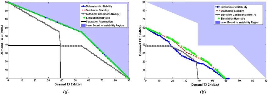
Fig. 4. Stochastic and deterministic stability regions, for a demand at Tx 1 of 0 Mb/s (a) and47.5Mb/s (b).
0 10 20 30 40 50 60 70 80 90 0 10 20
30 40 50 60 70 80
90 0
10 20 30 40 50 60 70 80 90
Demand TX1 (Mbps)
Demand TX2 (Mbps)
Demand TX
3
(Mbps)
(a) Stochastic stability region
0 10 20 30 40 50 60 70 80 90 0 10
20 30 40 50
60 70 80 90 0
10 20 30 40 50 60 70 80 90
Demand TX1 (Mbps) Demand TX2 (Mbps)
Demand TX
3
(Mbps)
(b) Deterministic stability region
0 10 20 30 40 50 60 70 80 90 0
10 20 30 40 50 60 70 80 90
Demand TX 1 (Mbps)
Demand TX
2
(Mbps)
0 5 10 15 20 25 30 35 40 45 50
(c) % Difference between stochastic and deter-ministic maximum rates for a transmitter, in func-tion of the arrival rates for the other two.
Fig. 5. Deterministic and stochastic stability regions, for the three node case.
0 5 10 15 20 25 30
0 0.2 0.4 0.6 0.8 1
λ(Mbps)
Av. Delay (ms) − TX
1 Model
Simulations
0 5 10 15 20 25 30
0 5 10 15 20 25
λ(Mbps)
Av. Backlog (Kb) − TX
1
Model Simulations
(a)
0 5 10 15 20 25 30
0 0.5 1 1.5 2
λ(Mbps)
Av. Delay (ms) − TX
2 Model
Simulations
0 5 10 15 20 25 30
0 20 40 60 80
λ(Mbps)
Av. Backlog (Kb) − TX
2
Model Simulations
(b)
0 5 10 15 20 25 30
0 50 100 150 200 250
λ(Mbps)
Av. Delay (ms) − TX
3 Model
Simulations
0 5 10 15 20 25 30
0 5000 10000 15000
λ(Mbps)
Av. Backlog (Kb) − TX
3
Model Simulations
(c)
Fig. 7. Mean delay and backlog (analytical vs simulation) whenλ1=λ;λ2= 1.5λ;λ3= 2λ: (a) Tx 1, (b) Tx 2, (c) Tx 3.
For comparison, we also plotted the stability region obtainable assuming a full saturated system, as well as the stochastic stability region derived by [7]. These plots show that our approach allows increasing sensibly the set of input rates for which the system is known to be stable, with respect to the well known stability region obtainable assuming coupling effects are always those of a saturated system. Such improvement is more marked the farther the system is from the saturation point.
1 2 3 4 5 6 10
20 30 40 50 60 70 80 90
# Users
Demand N−th Transmitter (Mbps)
Stochastic Stability Simulation Heuristic
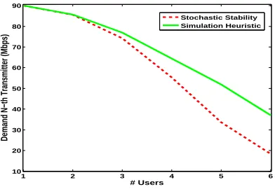
Fig. 6. Maximum demand of the N-th user for which the system is stochastically stable, as a function of N. The demand of all other users is
10Mb/s.
regression test to existing results for two nodes CPS, as discussed in Section IV. As those conditions are tight, they define a region (shadowed in the plots) for which the system is known to be unstable. Note that [7] performs well only when the demands of allof the nodes is under the saturation point. Indeed by [7] any point for which the demands of two or more nodes are above saturation is to be considered unstable. Such approach is therefore not efficient if the number of nodes in the system increases, because the probability of having a stable set of demands where the demands of two or more queues is above the demand that can be satisfied under saturation increases.
In order to have an indication of the tightness of our sufficient conditiond for stability we have run some simulations assuming Poisson arrivals, and observed the evolution over time of queue lenght at nodes for arrival rates in the interval
[0, Cmax]. For each combination of arrival rates, we have adopted the following crude heuristic in order to individuate system configurations which could be associated to instability. We have divided the simulation time (one hour) into five intervals, discarding the first in order to reduce the effect of initial transient. For each of the remaining intervals, we have computed the average queue length over the time interval. A set of rates has been considered as likely to lead to instability when, for at least one node, such average queue length increased steadily over the four intervals. As we can see from Fig. 4, the border of the region individuated by such heuristic are very close to the borders of the stochastic stability region given by our sufficient conditions. Such empirical estimations suggest that our conditions are reasonably tight, and that the set of arrival rates for which queues do not explode in practice is not much larger than the one individuated by our bounds.
In Fig. 5 we show the surface plot of the stochastic and the deterministic stability regions, both derived by optimizing the bounds in Sections IV-A and IV-B over the scaling values. As such bounds are based on different assumptions on input traffic, and as they relate to different notions of stability, in general they are not comparable. We can get an idea of their relative performance by considering the special case of leaky bucket constrained traffic sources, with leaky bucket rate ρ
equal to their mean traffic arrival rate. To a system with such input traffic characterization, we can apply both Theorem 4.1 for its stochastic stability, and Theorem 4.2 for its deterministic stability. Fig. 5 (but also Fig. 4) show that our stochastic stability conditions are looser than those for deterministic
stability, particularly around the saturation point. The mean relative difference is9.17%, with the bounds for deterministic stability being always tighter than those for stochastic stability. In order to have an idea of how the performance of our bounds change with respect to the number of nodes of the CPS, we have evaluated numerically the stochastic stability region for N ∈ 1, ...,6. For every value of N, we have set the demand of N−1 transmitters to 10 Mb/s, and we have computed the maximum demand of the N-th user for which the system is stochastically stable, according to our bounds, as well as the one resulting from our heuristic on simulations.
Fig. 6 shows that the difference between our bounds and simulation results increases with N. Indeed, our analysis is based on a worst case model of the behavior of each node. As our analysis is based on the feed forward structure of the upper bounding networks, the effects of the worst case approach cumulate at each stage, bringing to results which are more conservative as N (and therefore the number of stages of the feed forward networks) increases.
Finally we have assessed numerically the results on mean delay and backlog at CPS queues of Section IV-A, optimizing them over the scaling values satisfying Eq. (3), for the case of N=3. In order to observe how mean delay and backlog evolve when the system approaches instability, we have chosen a fixed (random) ratio between the demands of the three transmitters, with each ratio individuating a specific linear trajectory in the three-dimensional space of user demands. Along such trajectories we have evaluated the mean delay and backlog from Section IV-A, as well as those resulting from simulations, using our previously described heuristic to determine when to stop simulating in the trajectory.
In Fig. 7 we show the results for the trajectory with the greatest gap between simulation and analytical values. Simulation values are averaged over20simulation runs. The demands are expressed in function of λ, with λ1=λ;λ2= 1.5λ;λ3= 2λ.
The plots show that simulation results are very close to analytical values, with the latters being always larger than the formers. This is expected, given that our results are based on a worst case approach. We also see that, as the trajectory does not pass from the saturation point, the increase of the mean delay and backlog with load is faster at one node (transmitter 3 in the considered trajectory) than at the others. Moreover, at this node the sharp increase in mean delay and backlog from simulations takes place very close to the border of the stability region given by Theorem 4.1. All this suggest that our sufficient conditions for stochastic stability, and our approach in general are reasonably tight.
VI. CONCLUSIONS
considered a simple interference-limited wireless scenario to exemplify our method, showing the tightness of our analytical bounds. The proposed method can be applied to a large number of wireless scenarios (e.g., 802.11 and LTE with or without D2D), but also to multiprocessor systems, to problems of resource allocation in data centers, and in general to all those systems modeled through CPS and for which simulation has been so far the main tool available for performance analysis.
REFERENCES
[1] S. C. Borst, O. J. Boxma, and P. R. Jelenkovic, “Coupled processors with regularly varying service times,” inINFOCOM, pp. 157–164, 2000. [2] S. C. Borst, M. Jonckheere, and L. Leskel¨a, “Stability of parallel queueing systems with coupled service rates,”Discrete Event Dynamic Systems, vol. 18, no. 4, pp. 447–472, 2008.
[3] B. Rengarajan, C. Caramanis, and G. de Veciana, “Analyzing queueing systems with coupled processors through semidefinite programming,”
INFORMS: Applied Probability Session, 2008.
[4] S. Borst, N. Hegde, and A. Proutiere, “Interacting queues with server selection and coordinated scheduling: application to cellular data net-works,”Annals of Operations Research, vol. 170, no. 1, pp. 59–78, 2009.
[5] G. Fayolle and R. Iasnogorodski, “Solutions of functional equations arising in the analysis of two server queueing models,” inPerformance, pp. 289–303, 1979.
[6] F. Guillemin and D. Pinchon, “Analysis of the weighted fair queuing system with two classes of customers with exponential service times,” inJournal of Applied Probability, 2004.
[7] T. Bonald, S. C. Borst, N. Hegde, and A. Prouti´ere, “Wireless data performance in multi-cell scenarios,” in SIGMETRICS, pp. 378–380, 2004.
[8] M. Jonckheere and S. C. Borst, “Stability of multi-class queueing systems with state-dependent service rates,” inVALUETOOLS, p. 15, 2006.
[9] J.-Y. L. Boudec and P. Thiran,Network Calculus: A Theory of Deter-ministic Queuing Systems for the Internet, vol. 2050 ofLNCS. Springer, 2001.
[10] C.-S. Chang, Performance Guarantees in Communication Networks. London, UK, UK: Springer-Verlag, 2000.
[11] A. K. Parekh and R. G. Gallager, “A generalized processor sharing approach to flow control in integrated services networks: the single-node case,”IEEE/ACM Trans. Netw., vol. 1, pp. 344–357, June 1993. [12] G. Fayolle and R. Iasnogorodski, “Two coupled processors: The reduc-tion to a riemann-hilbert problem,”Zeitschrift fur Wahrscheinlichkeits-theorie und Verwandte Gebiete, vol. 47, no. 3, pp. 325–351, 1979. [13] G. Fayolle, Topics in the constructive theory of countable Markov
chains. Cambridge university press, 1995.
APPENDIX
A. Proof of Theorem 3.1
We begin with the following result, which defines a suffi-cient condition for a class of networks to upper bound a CPS:
Lemma A.1 (Upper Bounding Network): Consider a net-work with N0 ≥ N queues, such that there is a one-to-one mapping between the queues of the CPS and a subset of N
queues of the network. The mapping is such that each queue
j in the subset has the same arrivals at any time t as its corresponding queue nj in the CPS. Let Rnj(t) and Rj(t)
be the service rates at time t, respectively, at queue nj and queuej. If at any time t≥0, for each queuenj of the CPS, it holds Rj(t)≤Rnj(t), then the network upper bounds the
CPS.
Proof:We prove that at any timet≥0, the lengthqnj(t)
of each queuenj of the CPS is always smaller than the queue lengthqj(t)of the corresponding queue in the network. If this is the case, a bound on the backlog of j also holds for the corresponding queue of the CPS, so that the partial stability of the network implies the stability of the CPS. We prove
qnj(t)≤qj(t)by contradiction. Assume thatt
∗is the smallest
time for whichqnj(t ∗)> q
j(t∗)holds. As arrivals are the same in both queues, this implies that at timet∗ a bitbof traffic has left queue j in the network, while is still being served at the corresponding queuenj of the CPS. Assume the last bit served before bat queuej has been served att∗−j in the network, and the last bit has been served at queue nj at timet∗−nj.
From the definition of t∗,t∗−j ≥t∗−nj. This it means
it exist an instant t0 ∈[t∗−nj, t
∗), whereR
nj(t
0)≤R
j(t0), which contradicts the assumptions.
Proof: [Theorem 3.1] Let us indicate with Oj(¯b(t)) =
Rupnj −Fj(¯b(t))the instantaneous service rate for fresh traffic
at the j-th GPS node. Then(4) can be written as
Oj(¯b(t))≤R0nj(t) =Rnj(¯b(t)) (12)
HereRnj(¯b(t))is the service rate of queuenjof the CPS when
the queues active at the CPS at timetareonlyall those which correspond to active queues for fresh arrivals at the network at timet. (12) ensures that the service rate of each queue for fresh traffic of the network is always inferior to the one of the correspondent queues in the CPS, when all active queues for fresh arrivals in the network are associated to active queues at the CPS.
We now prove that such property is sufficient for the net-work to respect Lemma A.1. That is, we prove that if (12) holds at any node and any time t ≥0, then Oj(¯b(t))≤Rnj(¯a(t))
for any node j and any timet≥0. In the following, indeed, we prove that ¯b(t)≥a¯(t)at any time t. If so, from (12), it follows that
Oj(¯b(t))≤Rnj(¯b(t))≤Rnj(¯a(t))
hence proving the theorem.
In the following, we prove that¯b(t)≥¯a(t)by contradic-tion. Considering that the arrivals are the same at the nodes of the network and at the corresponding queues of the CPS, we can assume that att= 0,¯b(t) = ¯a(t).
Then, we assume by hypothesis that t∗ is the first moment where a queue nk that is not empty at the CPS turns empty in the corresponding node k of the network. In other words,
t∗ is the first moment where ¯b(t) ≥ ¯a(t) does not hold. In order to satisfy the hypothesis¯bk(t)<a¯nk(t), it exists at least
a moment t0 ∈ [0, t∗) where Ok(¯b(t)) > Rnk(¯a(t)). Since
the CPS is monotonic, this is possible just if at t0 one of the queues for fresh traffic is empty at the network, while the corresponding queue at the CPS is not. The existence of t0
contradicts the definition of t∗, proving the theorem.
B. Proof of Theorem 4.1
By applying Bayes’ result, and exploiting the independence between arrival processes, we have that∀j,
P(¯b(j−1)) =
j−1
Y
k=1
, whereP(bk)is the probability that the queue at thek-th stage is in state bk. We now prove Theorem 4.1 by induction.
First step:At the first stage, fresh traffic is served at a constant rate equal toRsat
n1 , as there are no endogenous arrivals. Hence
the sufficient condition for stability of that queue is λnj ≤
Rsat n1 =R
up
n1. At the second stage of network(¯n, ¯
S), when the queue for fresh traffic at the first stage is active, the arrival rate of traffic from the first stage isβ1=Rnup1 =R
sat n1. Hence,
from the structure of stage 2, the traffic in input to the policer is given byb1S2,1Rsatn1. As the policer at stage 2 has policing
rate Rup n2−R
sat
n2, the mean interfering rate at stage 2 is given
by
P(b1)·min(S2,1Rsatn1, R
up n2−R
sat n2)
P(b1)is equal to the mean utilization at node 1, which is given
by λn1
Rsat n1
. Finally, by the node stability condition at the queue for fresh traffic at node 2, the mean arrival rate must be not larger than the mean service rate for fresh traffic at that node. Given that the GPS node works at the fluid limit, the service rate for fresh traffic is equal to the minimum service rate dedicated to fresh arrivals, Rsat
n2, plus the part of service
which is not consumed by the endogenous traffic, which is given by Rup
n2 − R
sat
n2 −E[F2]. We have therefore that λn2≤R
up
n2−E[F2].
Induction step. We first note that for a given¯b(j−1), the arrival
rate at the policer of stage j is Pj−1
k=1Sj,kbkE[βk]. Hence, the rate impairment at stage j, for a given ¯b(j−1), is the min
between the arrival rate at the policer and the policing rate. The average rate impairment at j is then computed by Eq. (6). In order to compute the probability that the firstj−1queues are in state ¯b(j−1), we can computeP(bk) as
λnk
Rupnk−E[Fk], i.e., as
the average utilization of the queue for fresh arrivals at stage
k. Since the GPS works at fluid limit, the average service rate reserved to fresh arrival traffic is Rsat
nj plus the fraction
of capacity reserved for the endogenous traffic that remains unused, i.e., Rup
nj −R
sat
nj −E[Fj]. Please not that E[Fj] is
always less than Rup nj −R
sat
nj due to the policer at stage j.
Finally, by imposing node stability at the fresh traffic queue we get expression Eq. (5).
C. Proof of Theorem 4.2
Theorem 4.2 can be proved by induction on the index j
of the stages of the feed forward network. Let us consider a network (¯n,S¯) associated to the given CPS, and satisfying Theorem 3.1. Let us consider stage j >1. As stages 1 to j-1 are stable, βk(t), k ∈ 1, ..., j−1 is constrained by a leaky bucket arrival curve with rate ρnk. Hence, from Eq. (3), the
rate impairment is constrained by a leaky bucket arrival curve, with rate equal to min(Rup
nj −R
sat nj ,
Pj−1
k=1ρnkSj,k). Eq. (9)
derives from imposing that the sum of the leaky bucket rates of all arrivals at the GPS node should be less than its total service rate Rup