Article
A Study of Tangerine Pest Recognition Using
Advanced Deep Learning Methods
Shuli Xing 1, Marely Lee 2,*
Center for Advanced Image and Information Technology, School of Electronics & Information Engineering, Chonbuk National University, Jeonju, Chon Buk, South Korea; [email protected]
* Correspondence: [email protected]; Tel.: +82-10-3611-8004
Abstract: To improve the tangerine crop yield, the work of recognizing and then disposing of specific pests is becoming increasingly important. The task of recognition is based on the features extracted from the images that have been collected from websites and outdoors. Traditional recognition and deep learning methods, such as KNN (k-nearest neighbors) and AlexNet, are not preferred by knowledgeable researchers, who have proven them inaccurate. In this paper, we exploit four kinds of structures of advanced deep learning to classify 10 citrus pests. The experimental results show that Inception-ResNet-V3 obtains the minimum classification error.
Keywords: pest recognition; Tangerine; advanced deep learning; minimum classification error.
1. Introduction
Tangerine is known for its fresh citrus taste and for being low in calories and high in nutrient content. According to a report by the US Department of Agriculture, a medium-sized tangerine contains 29.1 mg of vitamin C, which supplies nearly 50% of daily requirement. It is well known that vitamin C is a powerful, natural, water-soluble antioxidant that can help the body resist infectious agents and eliminate cancer-causing free radicals [1]. In addition, Tangerines are rich in potassium and low in sodium. This contributes to the relaxing of blood vessels and maintenance of proper blood pressure. However, due to the effects of several citrus pests, the quality and quantity of tangerines has been significantly reduced. In order to control the citrus pests, two types of approaches are commonly adopted: a biological control method and a chemical pesticides control method. No matter which method is chosen, monitoring and identify a species of citrus pest in time can greatly help in reducing yield loss. In this paper, the recognition tasks are based on the features extracted from images that have been collected from websites and Jeju Island (South Korea) tangerine plantations.
For low-dimensional data, using conventional classification algorithms, such as k-nearest-neighbor (KNN), support vector machine (SVM), and multilayer perceptron (MLP), is reasonable. Even though for a new input dataset we cannot employ transfer learning to fine-tune the trained model, these traditional algorithms are so computationally simple that they are not time-sensitive, and the hyper-parameters in them that need to be considered are few, compared with deep learning. However, as for high-dimensional data (for example, when the input image size is 224 × 224), the performance of algorithms mentioned above are not as good as that of convolutional neural networks (CNNs), although some preprocessing techniques—for example, principal components analysis (PCA) can be used for reducing the redundancy of input. A research about image classification problem was conducted in [2], which compares the accuracy of KNN, SVM, and MLP with that of CNNs. In terms of 10 labeled datasets, CNN (Inception-V3) with transfer learning gets the highest classification accuracy (88%), CNN-2 (there are two convolutional layers and two fully connected layers in total) without transfer learning second (43.1%). The worst was SVM, with an accuracy < 0.1%.
The development of CNN has dramatically improved the state-of-the-art in computer vision and natural language processing [3]. In general, one kind of CNN is composed of four parts: convolutional
layer, pooling layer, activation function, and fully connected layer. Apart from these basic components, the batchnormalization layer [4] and dropout layer [5] are always added to overcome the problem of local gradient vanishment and overfitting.
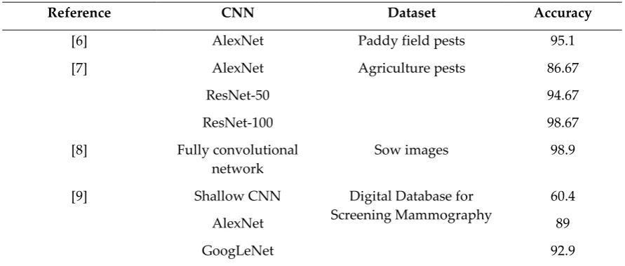
CNN models can be applied to many domains, such as agriculture, stockbreeding, and medical treatment (refer to Table 1). This phenomenon gives us the confidence to apply this technology for tangerine pest recognition. We explored four kinds of structures of advanced deep learning: VGG, Residual Network, Inception modules, and Xception. They have achieved great success and other recent models are almost their variants. The experimental results show that Inception-ResNet-V3 gives the best classification performance.
Table 1. The related works use CNNs as classifiers.
Reference CNN Dataset Accuracy
[6] AlexNet Paddy field pests 95.1
[7] AlexNet
ResNet-50
ResNet-100
Agriculture pests 86.67
94.67
98.67
[8] Fully convolutional network
Sow images 98.9
[9] Shallow CNN
AlexNet
GoogLeNet
Digital Database for Screening Mammography
60.4
89
92.9
Our paper is structured as follows. Section 2 describes the dataset for classification. Section 3 discusses the strengths and weaknesses of the four selected structures. In Section 4, we present our experimental results and compare the performance of these algorithms. Section 5 contains the conclusion and discusses future work.
2. Dataset
2.1. Tangerine Pests Description
Asian citrus psyllid (ACP) is regarded as a key pest because it is a carrier of huanglongbing (HLB), which is the most destructive disease in citrus-growing areas worldwide. HLB causes asymmetrical blotchy mottling of leaves. Fruit from HLB-infected trees is of no value because of poor size and quality [10].
Stink bugs are well known “plant feeders”. They attack fruits, vegetables, and ornamental plants. Many species of stink bugs have been found feeding on citrus, and their favorite citrus seems to be the tangerine. The southern green stink bug (SGSB) is the one that attacks citrus most frequently [11]. When the SGSB punctures a piece of citrus, it leaves hard brownish or black spots. These injuries influence the citrus’ edible qualities and, thus, lower its market value.
Asian longhorned beetle (ALB) is also a serious pest of citrus. China, Japan, and Korea are considered to be its origins. However, with the increase in global trade and movement of wood packing material, ALB is now found in more than 19 countries in the world [12]. The damage caused by the adult ALB is minor, but larval tunneling in the cambial region and the wood is deadly to citrus trees because it hinders the water and nutrient transportation.
Besides the four major pests described above, citrus swallowtail (CS), fork-tailed bush katydid (FTBK), green leafhopper(GL), Chinese fruit fly(CFF), fruit-piercing moth(FPM), and citrus mealybug (CM) are all picked as labels of the deep learning models. Each pest’s representative pictures are shown in Figure 1.
Figure 1. The sampling pictures for each kind of pest.
2.2. The Image Data of Tangerine Pests
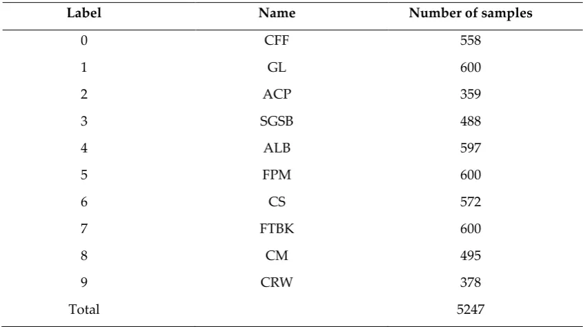
A total of 5247 images are included in our dataset (refer to Table 2). In the same pest folder, the similarity of every two images is lower than 80%, which enhances the diversity of sampling. The size of all images is resized to 224 × 224 by a bilinear interpolation approach during training and testing. According to the statistical results in [13], we guarantee that the scale of object to be recognized in the image is higher than 50%.
Table 1. The list of species and number of samples for the pest recognition.
Label Name Number of samples
0 CFF 558
1 GL 600
2 ACP 359
3 SGSB 488
4 ALB 597
5 FPM 600
6 CS 572
7 FTBK 600
8 CM 495
9 CRW 378
Total 5247
Furthermore, in order to strengthen the robustness of pest recognition, two measures have been taken:
The effect of viewing angles on insect identification has been discussed in [14], which encouraged us to gather the pest photos with diverse shooting angles. Take the ALB as an example. The same ALB photographed at different angles shows different patterns (refer to Figure 2). This strong view dependence may lead to incorrect classification for CNNs with single-angle inputs.
Figure 2. ALB images with different viewing angles.
• The backgrounds of images are varying
Compared with indoor conditions, the visual noise of natural environments is more complicated and uncontrollable. In the early literature of pest detection [15-16], in order to reduce the impact of visual noise on recognition accuracy, some image segmentation algorithms were used to capture the desired objects from cluttered backgrounds. However, there are still unstable factors that affect the performance of these approaches—for example, the selection of thresholding for pixels and histogram [17]. When the pest’s camouflage has the same appearance as its surroundings (refer to Figure 3), the image segmentation methods seem to be invalid.
On the other hand, increasing the background complexity of images can boost the generalization of CNNs. Overfitting is universal in machine learning, and it is caused by inadequate learning from training examples. The simplest way to avoid this problem is to diversify the types of samples. The varying background is an obstacle to setting threshold values for segmentation algorithms, but here it impairs the correlation between two images.
(a) (b) (c)
Figure 3. The images of citrus pests whose cryptic colorings are the same as those of their surroundings: (a) is GL, (b) is SGSB, and (c) is larvae of CS.
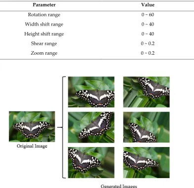
2.3. Data Augmentation
Another effective way to help the model generalize is data augmentation (DA). In fact, the field of DA is not new, and various techniques of it have been applied to specific problems [18-19]. The generic practice in augmenting image data is to perform geometric transformations, such as rotation, reflection, shift, flip, etc.
The influence of unbalanced data on classification performance has been discussed in [20], which prompted us to increase the number of images of pest whose dataset scale is smaller than that of others. An example of images generated by random combinations of geometric transformations is shown in Figure 4. Table 3 gives the parameter set of transformations. After the DA operations, each type of pest contains 600 images.
Data Augmentation
Parameter Value
Rotation range 0 ~ 60
Width shift range 0 ~ 40
Height shift range 0 ~ 40
Shear range 0 ~ 0.2
Zoom range 0 ~ 0.2
Figure 4. Original image and generated images by DA
3. Advanced Deep Learning Models
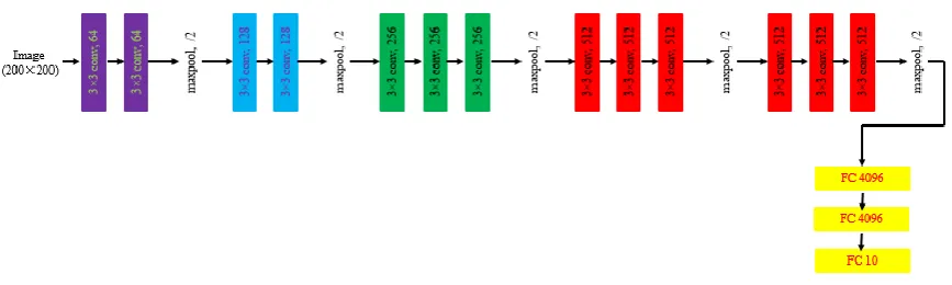
Convolutional filters have been used for many years to extract features from 2D shapes. The first successful structure of CNN is LeNet-5, which applied gradient-based learning to update weights and biases [21]. The use of LeNet-5 has considerably reduced the test errors of handwritten digit recognition from 12% to 0.8%. Based on GPU implementation, AlexNet [22] greatly increased the depth of LeNet-5, and this architecture also won the first prize in the 2012 ImageNet competition. The design of the VGG model makes the structure of CNN deeper and wider.
3.1. VGG
There are three main factors that contribute to improving the performance of CNN: • Depth: the number of convolutional layers
• Width: the number of convolutional filters in each layer • Better utilization of model parameters
same computational resource to construct a deeper CNN model. For example, one 5×5 convolutional layer can be replaced by two layers of 3×3 convolution. Moreover the parameters of two 3×3 convolutional layers is 1.39 times less than that of one layer of 5×5 convolution.
Figure 5. The configurations of VGG – 16
3.2. Residual Network
It is generally believed that the deeper network construction, the higher the classification accuracy that will be derived. However, as the depth of the CNN increases, the accuracy gets saturated and then drops rapidly. The design of residual networks (RN) is aimed at solving the problem of degradation [24]. Instead of directly fitting a desired underlying mapping, He et al. [25] adds an identity mapping to each building block. To save computation costs, two layers of 1×1 convolution are embedded in residual block (refer to Figure 6). The first 1×1 convolution is used for reducing the computation complexity, and the second layer of 1×1 convolution is responsible for increasing the dimensions. The same bottleneck architecture is followed in this paper.
(a) (b)
Figure 6. (a) is residual block without 1×1 convolution layers; (b) is bottleneck architecture with two layers of 1×1 convolution. Structure (a) it needs 589825 (256*3*3*256) float points. The computation cost of structure (b) is 69632 (256*1*1*64 + 64*3*3*64 + 64*1*1*256). With regard to depth, architecture (b) is three times deeper than (a).
The invention of Inception models breaks the mode of stacking layers, which provides us with a new way to increase the depth and width of a CNN. Inception models are more difficult to design than a VGG or RN because of the diversified modules in them. However, under the same computational budget, Inception models can be constructed more deeply and widely so as to achieve more accuracy than a VGG or RN.
There have been four generations of the Inception model: Inception-V1 [26], Inception-V2 [4], Inception-V3 [27], and Inception-V4 [28]. Among these, Inception-V1 is the simplest, and it is a practical model designed by Arora et al. [29]. Inception-V2 replaces the 5×5 convolutional layers of Inception-V1 with two consecutive 3×3 convolutional layers. Inception-V3 and inception-V4 adopt asymmetric convolutions to further increase depth, but the former has fewer model parameters.
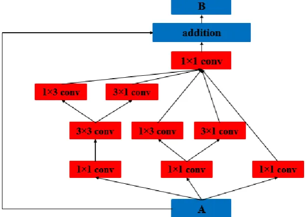
According to the above comparison, Inception-V3 is selected as the basic model. Meanwhile, we also added identity mapping to each module of it to accelerate the training speed. Figure 7 shows one of the modules in the improved Inception-V3 (Inception-ResNet-V3).
Figure 7. An example of module in Inception – ResNet – V3: A and B are groups of feature maps.
3.4. Xception
(a) (b)
Figure 8. (a) is regular convolution, (b) is separable convolution. Suppose the input channels of (a) and (b) are both m and output channels are both u. Then the number of parameters involved in calculation of (a) is m*3*3*u, and that of (b) is m*3*3 + m*1*1*u.
Figure 9. An example of building block in Xception. Here, the 1×1 convolution is used for downsampling because stride = 2×2.
4. Experiment and Results
In this section, the first four parts represent the preparations for training models. The last part compares different aspects of the selected architectures.
4.1. Experiment Setup
We randomly selected 500 images from each pest folder to train models and the ratio between training set and validation set is 4:1. The remaining 100 images were used for testing. The framework used to implement the models is Keras with TensorFlow for the backend. The hardware foundation is GPU (GTX 1080Ti, 12G). The code and models are available at https://github.com/xingshulicc/citrus-pest-classification-by-advanced-deep-learning.
4.2. Hyperparameters of Models
Besides the structure, the hyperparameters of the model can also determine the performance of the classification.
• Mini-batch size
The most popular algorithm for updating weights and biases of deep neural networks is the mini-batch stochastic gradient descent (SGD). Therefore, a good choice of mini-batch size can help improve the quality of the models. In theory, a large batch size can better approximate the statistics of entire dataset and, thus, increase the convergence precision. However, Masters et al. [33] have proven that the small values of batch size (between 2 and 32) sped up training and enhanced model generalization capability. Based on the experimental results of [33], we selected 8 as the final batch size.
• Learning rate
A static learning rate may lead to slow convergence or fluctuation around the minimum. Thus, we hoped that the learning rate could be changeable during training. The learning rate was initialized with 0.0001, and a decay (10-5) was introduced to reduce the value of the learning rate for every epoch.
• Momentum
Momentum contributes to accelerating convergence, and its value is usually set to 0.9. There are two types of momentum in deep learning: classical and Nesterov [34]. Nesterov momentum has recently become a preferred choice because it can change the velocity of gradient descent in a quicker and more responsive way.
4.3. Transfer Learning
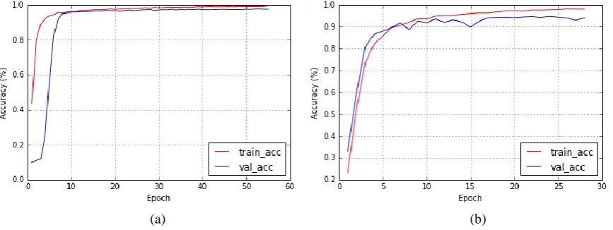
Transfer learning allows us to transfer the knowledge gained from one problem to a different but related problem. It significantly promotes the efficiency of learning. A good example of transfer learning for CNNs is the initialization with a pre-trained model. Moreover, Yosinski et al. [35] have found that the convolutional filters in different depths play distinct roles. In the first-layer convolutions, extracted features are general and can be applicable to other datasets. However, the features learned from convolutional layers that are close to the classification layer are not general but specific.
Figure 10. (a) VGG-16 with pre-training; (b) is VGG-16 without pre-training. The red curve in (a) and (b) is training accuracy, and the blue curve is validation accuracy.
4.4. Against Overfitting
In fact, even though the model has been pre-trained, we notice that the problem of overfitting still exists (refer to Figure 10a). Overfitting cannot be completely eliminated but can be reduced to a low level by available methods. Besides the extension of the dataset, decreasing the complexity of model is an alternative method.
The number of parameters in fully connected layers usually accounts for half of the total parameters of the networks. Therefore, restricting the size of fully connected layers becomes a priority. In general, dropout [5] is the first choice. This approach drops units from the neural network during training by multiplying the Bernoulli distributed random variables. This method produces many potential subnetworks in the period of training. At test time, to approximate the effect of these thinned networks, their average predicted number is calculated. However, it has been proven that the dropout can slow down the speed of training. Another available method is global average pooling (or global max pooling), which was first proposed in network in network [36]. The global average pooling layer computes the average of each feature map from the last convolutional layer and feeds the average values directly into the classification layer. Global average pooling saves more time per epoch than dropout (refer to Table 4). The structures of fully connected layers constructed by dropout and global average pooling are shown in Figure 11.
(a) (b)
Early stopping is able to work against overfitting but not by altering the complexity of the model. It enables us to monitor the error in the validation set and stop the training if improvement in the error rate does not occur in a timely manner.
Table 4. The time consumption per epoch and total parameters of networks with different fully connected layers.
VGG-16
Time (s) / epoch Total Parameters (float)
Dropout 61 107,038,538
Global Average Pooling 44 14,982,474
According to the comparison as shown in Table 4, we give preference to global average pooling with early stopping. The patience of early stopping is defined as follows:
if the validation error at epoch n is minimum:
then stop training after 5 epochs
4.5. Classification Performance and Comparisons
The training results of selected models with early stopping are shown in Figure 12. It can be seen that the overfitting in each model has been controlled at a very low degree (< 4%). With regard to convergence, VGG-16 is the fastest. It stopped at 28 epoch with 98.12 training accuracy and 94.05 validation accuracy. On the contrary, the convergence of Xception is the slowest, which stopped at 100 epoch but with higher training and validation precision.
As for computational complexity (refer to Table 5), Inception-ResNet-V3 occupies the most computing resources, with 54,352,106 parameters in total. ResNet-50, composed of 27,804,554 parameters, ranks second. The least one is VGG-16, which only has 14,982,474 parameters. Another interesting finding displayed in Table 5 is that the time consumption per epoch of Xception is larger than that of ResNet-50 and Inception-ResNet-V3. The reason for this is that the identity mappings in ResNet-50 and Inception-ResNet-V3 accelerate the speed of training.
(c) (d)
(e)
Figure 12. The training process of the four models mentioned previously: (a) is ResNet-50 (b) is VGG-16 (c) is Inception-ResNet-V3 and (d) is Xception; (e) is their final training performance.
Table 5. The computational complexity and time consumption per epoch of each model.
Model
VGG-16 Xception ResNet-50 Inception-ResNet-V3
Total Parameters
14,982,474 25,078,322 27,804,554 54,352,106
Trainable Parameters
14,943,754 25,022,866 27,741,834 54,290,666
Non-trainable Parameters
38,720 55,456 62,720 61,440
Time (s) / Epoch
44 60 44 58
According to Table 6, we find that the more complexity with which a network is constructed, the better classification performance it achieves. For example, the test accuracy of Inception-ResNet-V3 is the highest, and VGG-16 gets the worst classification result, unsurprisingly. This phenomenon is also consistent with the strategies used to improve the performance of CNNs.
Table 6. The test performance of each model.
Model Accuracy (%)
98.12
99.53 99.04 98.27
94.05
97.58 98.79 98.19
91 92 93 94 95 96 97 98 99 100
VGG-16 RESNET-50 INCEPTION – RESNET – V3 XCEPTION
Training Performance
VGG-16 94.01
Xception 98.25
Inception – ResNet – V3 98.73
ResNet – 50 97.62
We have analyzed the confusion matrix of Inception-ResNet-V3 for the test dataset (refer to Table 7) and found that the error rate of CRW is the highest (6%). The misclassified images are shown in Figure 13. Different species of pest can present similar shape and color pattern under special shooting conditions. The probability of this case is very low but inevitable in the process of data collection. Inception-ResNet-V3 performed badly on identification of these samples, which proved that the model produced divergence on the classification of fine-grained images.
Figure 13. The misclassified samples in the test dataset.
CS FTBK GL CRW CFF FPM CM SGSB ACP ALB
CS 100 0 0 0 0 0 0 0 0 0
FTBK 0 100 0 0 0 0 0 0 0 0
GL 0 0 98 0 0 0 0 1 1 0
CRW 0 1 0 94 2 0 0 1 1 1
CFF 0 0 0 0 99 0 0 0 0 1
FPM 0 0 0 0 0 100 0 0 0 0
CM 0 0 0 0 0 0 99 1 0 0
SGSB 0 0 1 0 0 0 0 99 0 0
ACP 0 0 1 0 1 0 0 0 98 0
ALB 0 0 0 0 0 0 0 0 0 100
5. Conclusions and Future Work
Because of pest damage, the quality and quantity of tangerines has been reduced. To improve the yield of this fruit, four types of CNN models were applied to identify species of citrus pests. We initialized the convolutional layers of each model by transfer learning method and freezing the parameters of the first convolutional layer during training and testing. However, we found that the overfitting problem was still considerable. Therefore, to reduce the level of overfitting, a global average pooling and early stopping approach were utilized. The experimental results show that Inception-ResNet-V3 got the highest classification accuracy (98.73 %) and the second shortest time per epoch (58s).
For the trained model, there are two serious problems need to be solved in the future (refer to Table 8):
1. It is difficult to store entire network architecture in a small computational budget device. 2. The runtime of different platforms is long.
Table 8. The comparison of running performance of Inception-ResNet-V3 on computer and smart phone.
Test Platform Model size Running time / image
Computer - GPU: GTX 1080Ti, 12 G
436.8 MB 14 ms
In addition, the disease in tangerines can also cause huge economic losses. Therefore, we are trying to collect image data of citrus diseases and select suitable CNN models to recognize them.
Author Contributions: Shuli Xing designed the study, performed the experiments and data analysis, and wrote the paper. Malrey Lee advised in the design of architectures and analyzed to find the best methods for tangerine pests recognition.
Acknowledgments: This work was supported by the National Research Foundation of Korea (NRF) granted by the Korea government (MSP) (No: 2017R1A2B4006667).
Conflicts of Interest: The authors declare no conflict of interest.
References
1. Liu, Y., Heying, E., Tanumihardjo, S. History, global distribution, and nutritional importance of citrus fruits. Comprehensive Reviews in Food Science and Food safety. 2012, 11, 530–545.
2. Image Classification with 5 methods. Available online: https://github.com/Fdevmsy/Image_Classification_with_5_methods (accessed on 10 May 2017).
3. LeCun, Y., Bengio, Y., Hinton, G. Deep learning. Nature. 2015, 521, 436–444.
4. Ioffe, S. and Szegedy, C. Batch normalization: Accelerating deep network training by reducing internal covariate shift. arXiv 2015, arXiv: 1502.03167.
5. Srivastava, N., Hinton, G., Krizhevsky, A., Sutskever, I., Salakhutdinov, R. Dropout: A simple way to prevent neural networks from overfitting. JMLR. 2014, 15, 1929–1958.
6. Liu, Z. et al. Localization and Classification of Paddy Field Pests using a Saliency Map and Deep Convolutional Neural Network. Sci. Rep. 2016, 6, 20410.
7. Cheng, X., Zhang, Y., Chen, Y., Wu, Y., & Yue, Y. Pest identification via deep residual learning in complex background. Computers and Electronics in Agriculture. 2017, 141, 351-356.
8. Yang, A., Huang, H., Zheng, C., Zhu, X., Yang, X., Chen, P., Xue, Y. High-accuracy image segmentation for lactating sows using a fully convolutional network. Biosystems Engineering. 2018, 176, 36-47.
9. Lévy, D., Jain, A. Breast Mass Classification from Mammograms using Deep Convolutional Neural Networks. arXiv 2016, arXiv: 1612.00542.
10. Baldwin, E., Plotto, A., Manthey, J., McCollum, G., Bai, J., Irey, M., Cameron, R., Luzio, G. Effect of liberibacter infection (Huanglongbing disease) of citrus on orange fruit physiology and fruit/fruit juice quality: chemical and physical analyses. J. Agric. Food Chem. 2010, 58, 1247–1262.
11. Hoffmann, M.P., Davison, N.A., Wilson, L.T., Ehler, L.E., Jones, W.A., Zalom, F.G. Imported wasp helps control southern green stink bug. California Agriculture. 1991, 45 (3), 20-22.
12. Hull-Sanders, H., Pepper, E., Davis, K., Trotter, R.T. Description of an Establishment Event by the Invasive Asian Longhorned Beetle (Anoplophora Glabripennis) in a Suburban Landscape in the Northeastern United States. PLoS ONE. 2017, 12(7), e0181655.
13. Russakovsky, O., Deng, J., Su, H., Krause, J., Satheesh, S., Ma, S., Huang, Z., Karpathy, A., Khosla, A., Bernstein, M., Berg, A. C., and Fei-Fei, L. ImageNet large scale visual recognition challenge. arXiv 2014, arXiv: 1409.0575.
14. Nguyen, C., Lovell, D., Oberprieler, R., Jennings, D., Adcock, M., Gates-Stuart, E., et al. Virtual 3D models of insects for accelerated quarantine control. In Proceedings of the 2013 IEEE International Conference on Computer Vision Workshops, Sydney, NSW, Australia, 2-8 Dec. 2013; pp. 161–167.
15. Boissard, P., Martin, V., Moisa, S. A Cognitive Vision Approach to Early Pest Detection in Greenhouse Crops. Computers and Electronics in Agriculture. 2008, 62, 81–93.
16. Faithpraise, F., Birch, P., Young, R., Obu, J., Faithpraise, B., Chatwin, C. Automatic Plant Pest Detection and Recognition Using k-means Clustering Algorithm and Correspondence Filters. Int. J. Adv. Biotechnol. Res. 2013, 4, 189–199.
17. Raju, P., Neelima, G. Image Segmentation by using Histogram Thresholding. IJCSET. 2012, 2(1), 776–779. 18. Mas Montserrat, D., Lin, Q., Allebach, J., Delp, E. Training object detection and recognition CNN models
using data augmentation. In Proceedings of the IS&T International Symposium on Electronic Imaging, Burlingame, California, USA, 29 January - 2 February 2017; pp. 27-36.
20. Ma, J., Du, K., Zheng, F., Zhang, L., Gong, Z., Sun Z. A recognition method for cucumber diseases using leaf symptom images based on deep convolutional neural network. Computers and Electronics in Agriculture. 2018, 154, 18-24.
21. LeCun, Y., Bottou, L., Bengio, Y., Haffner, P. Gradient-based learning applied to document recognition. Proc. IEEE. 1998, 86 (11), 2278–2324.
22. Krizhevsky, A., Sutskever, I., Hinton, G.E. ImageNet classification with deep convolutional neural networks. In NIPS, 2012; pp. 1097–1105.
23. Simonyan, K., Zisserman, A. Very deep convolutional networks for large-scale image recognition. arXiv 2014, arXiv: 1409.1556.
24. He, K., Zhang, X., Ren, S., Sun, J. Deep residual learning for image recognition. arXiv 2015, arXiv: 1512.03385.
25. He, K., Zhang, X., Ren, S., Sun, J. Identity mappings in deep residual networks. arXiv 2016, arXiv: 1603.05027.
26. Szegedy, C., Liu, W., Jia, Y., Sermanet, P., Reed, S., Anguelov, D., et al. Going deeper with convolutions. arXiv 2014, arXiv: 1409.4842.
27. Szegedy, C., Vanhoucke, V., Ioffe, S., Shlens, J., Wojna, Z. Rethinking the inception architecture for computer vision. arXiv 2015, arXiv: 1512.00567.
28. Szegedy, C., Vanhoucke, V., Ioffe, S. Inception-v4, inception-resnet and the impact of residual connections on learning. arXiv 2016, arXiv: 1602.07261.
29. Arora, S., Bhaskara, A., Ge, R., Ma, T. Provable bounds for learning some deep representations. In Proceedings of the 31st International Conference on Machine Learning, Beijing, China, June 21 – 26 2014; pp. 584–592.
30. Chollet, F. Xception: Deep learning with depthwise separable convolution. arXiv 2016, arxiv: 1610.02357. 31. Howard, A.G., Zhu, M., Chen, B., Kalenichenko, D., Wang, W., Weyand, T., Andreetto, M., Adam, H.
Mobilenets: Efficient convolutional neural networks for mobile vision applications. arXiv 2017, arXiv: 1704.04861.
32. Sandler, M., Howard, A., Zhu, M., Zhmoginov, A., Chen, L.-C. Inverted residuals and linear bottlenecks: Mobile networks for classification, detection and segmentation. arXiv 2018, arXiv: 1801.04381.
33. Masters, D., Luschi, C. Revisiting Small Batch Training for Deep Neural Networks. arXiv 2018, arXiv: 1804.07612.
34. Sutskever, I., Martens, J., Dahl, G. E., Hinton, G. E. On the importance of initialization and momentum in deep learning. In Proceedings of the 30th International Conference on Machine Learning (ICML-13), Atlanta, GA, USA, June 16 – 21 2013; pp. 1139–1147.
35. Yosinski, J., Clune, J., Bengio, Y., and Lipson, H. How transferable are features in deep neural networks? In NIPS, 2014; pp. 3320–3328.