Effects of Multiple Behavioral Drivers on Collective Conservation Outcomes

(1)

1

Title: Effects of multiple behavioral drivers on collective conservation outcomes

Authors: Yletyinen, J.1,2_{*, Perry, G.L.W.}3_{, Brown, P.} 4_{, Pech, R.}2_{, Tylianakis, J.M.}1

Affiliations: 1. University of Canterbury, School of Biological Sciences, Private Bag 4800, Christchurch 8140, New Zealand

2. Manaaki Whenua - Landcare Research New Zealand Ltd., PO Box 69040, Lincoln 7640, New Zealand

3. School of Environment, University of Auckland, Private Bag 92019, Auckland, New Zealand

4. Manaaki Whenua - Landcare Research New Zealand Ltd., PO Box 10345, Wellington 6011, New Zealand

*) corresponding author: [email protected]

Abstract

Conservation of natural habitats in human-dominated landscapes is critical for halting biodiversity loss. Maintaining habitat quantity and connectivity requires landscape-level collective action, which results from environmental decisions made by individual land owners. We investigate how individual decision making in a rural collective translates into quantitative differences in landscape-level environmental outcomes. Behavioral science has become a critical domain of knowledge in conservation, but little attention has been paid to how multiple behavioral drivers determine the success of collective environmental action. We developed a social-ecological model for landscape-level conservation using a detailed data set of 600 land owners in New Zealand. With the model, we tested whether the effect of social influence networks on collective conservation action was altered by their interplay with land owners’ personal characteristics, connections to cross-scale actors and local

environmental contexts. Interactions between multiple behavioral drivers determined the environmental outcomes of collective action in unexpected ways by modifying, muting or amplifying the effects of single drivers. Importantly, we detected a social-ecological mechanism for rapid change in the extent of protected habitats, which can explain highly successful or failed environmental outcomes of collective conservation. Further, when environmentally desirable and undesirable behaviors spread simultaneously through the

(2)

2

social network, homophily and network cohesion hinder desirable environmental outcomes. This effect can be modified by other drivers such as social responses to local environmental change. Thus, understanding how the antagonistic and synergistic effects of behavioral drivers can be best utilized in conservation will benefit biodiversity and ensure benefits that humans obtain from biodiversity.

Key words: pro-environmental behavior, social-ecological systems, conservation, social networks, landscape structure

Plain-language abstract:

Biodiversity conservation efforts frequently depend on local land owners’ participation. However, critical knowledge gaps remain in understanding how individual behaviors collectively lead to desired environmental change. Using an empirically informed social-ecological model for landscape-level conservation, we show that mechanisms emerging from the interplay of behavioral drivers can lead to accelerating environmental change and that effects of single drivers depend on the influences of other drivers. In the context of land owners who vary in their values and relationships, an interplay between behavioral drivers can explain unexpected outcomes of collective conservation, including failure to achieve environmental change. Hence, the benefits of behavioral insights for the success of conservation initiatives depend on better understanding of the ways in which behavioral drivers interact.

Halting global biodiversity loss requires increases in protected areas and efficiency of

conservation efforts (1). Protecting native or semi-natural habitat patches on agricultural land can sustain local biodiversity and provide habitat connectivity between existing protected areas (2, 3). Agricultural land covers circa 37 per cent of global terrestrial area, and

humanity’s demand for food, biofuels and fibre is increasing, placing further strain on natural habitats (4–6). Land-use decisions made by individual land owners are thus pivotal in

(3)

3

Conservation is most effective when individuals who have adopted pro-environmental behavior influence broader systems such as social networks and social norms (9–11). Therefore, understanding how the environmental behavior of individuals leads to a system-wide change iscrucial for achieving environmental change. A substantial body of literature has considered what motivates individuals to participate in voluntary conservation (12). However, much less is known about why formal or informal collective behavior emerging from individual behaviors in some cases succeeds, and in others fails, in effecting

environmental change (10, 13).

Here, we examine how mechanisms emerging from theinterplay between multiple constraints and drivers of pro-environmental behavior influence collectively achieved

environmental change. The spread of pro-environmental behavior is driven by factors such as social network structure (14)andpersonal characteristics (15). However, it is likely that multiple ecological and social behavioral drivers interact in complex ways to influence environmental outcomes (10, 16), and such interactions cannot be revealed by studies focusing on single drivers (11). To investigate the effects of multiple behavioral drivers, we ask how the effect of social-influence networks on conservation outcomes in agricultural landscapes is modified by cross-scale social influences, actor attributes and local

environmental change. We relax the common assumption that influence and behaviors almost inevitably spread between connected individuals (e.g. 14, 17 and references within), and instead assume that: i) behavioral decisions are affected by multiple drivers, and ii) both environmentally desirable and undesirable behaviors1 can simultaneously spread through a social network (18, 19). Peer influence (i.e. social network connectivity) between land

owners can generate desired or undesired environmental behavior and, consequently, patterns of social influence among land owners may determine landscape structure. The propensity of land owners to associate with and be influenced by other like-minded land owners (a process termed ‘homophily’ [20, 21]) can thus generate socially (but not necessarily spatially) aggregated behaviors. Conversely, social norms and behavior may be transmitted locally (“I see others do it, so it must be a good thing to do”) through changes in natural areas, for example among neighboring properties (22, 23). The local influence of social norms on behavior would, therefore, tend to generate spatially aggregated clusters of similar

1_{We use the terms “desirable” and “undesirable” from a biodiversity-conservation perspective. Thus,}

(4)

4

behavior(s). The spread of pro-environmental behavior is especially important in natural habitat conservation because biodiversity is strongly influenced by the composition,

abundance and spatial configuration of habitats at the landscape level (hereafter, ‘landscape structure’) (24).

While social structures profoundly impact collective environmental action (see discussion on drivers below), their effects on environmental change are rarely measured (13). We

implement a social-ecological agent-based model (Figure 1) to explore how individual decision-making in a rural collective translates into differences in landscape-level native forest conservation. The model is based on survey data of 600 New Zealand land owners that included questions on land use practices, sources of environmental information and personal characteristics (for a summary of the survey methods and general results, see [25]). New Zealand provides an ideal context to explore the emergence of natural habitat conservation on agricultural land: agricultural land covers 42 per cent (in 2015) of the land area (4), and although protecting native habitat on agricultural land is voluntary in New Zealand, the agricultural sector is under societal pressure to improve its environmental performance while maintaining its position as New Zealand's largest sector of tradable goods (26).

Our study includes the following four types (i – iv) of behavioral drivers. First, behavioral science suggests that each person has a set of personal characteristics and beliefs influencing his or her decisions about participation in environmental action (9), which are called (i) actor attributes when associated with social networks. Much empirical research has sought to identify the predictors of land owners’ adoption of conservation practices (15). A suite of universal predictors has not been identified; instead, they are likely to be context-dependent (15).

Further, behavior, information and ideas spread through (ii) social networks as individuals’ opinions are weighted in relation to those of others per social influence network theory (27).

Threshold models of collective action show that an individual's adoption of a behavior is influenced by the number of people already practicing that behavior and their susceptibility to influence (28). We include network link weights to capture the self-reported level of

(5)

5

networks (29). The importance of the effect of homophily in collective action has been acknowledged, but its effect on collective behavior is not fully understood (21).

The third behavioral driver we consider is (iii) cross-scale groups, i.e. social actors who do not directly modify the environment but who may influence other actors to do so, thereby indirectly affecting environmental outcomes (30). Communication between cross-scale actors and local land owners can shift perceptions of conservation and so enhance and coordinate local environmental action (31). Due to their ability to influence environmental chance, we include three cross-scale groups in the experiments and assume them to be

pro-environmental. We include two stakeholder groups and one indigenous group but discuss them as one driver.

Finally, humans use the behavior of others to guide their own actions and are generally reluctant to deviate from social norms (32). Consequently, observable cues of widespread support for environmentally desirable action can change behaviors (11, 33). Since both macro-level environmental and social dynamics arise from micro-level social (or social-ecological) interactions (34), local environmental change or reductions in collective behaviors can erode a social norm or affect opinions, ultimately leading to a cascading change in behavior (35, 36). To represent how environmental changes resulting from

individual actions feed back to influence future environmental decisions, we include a fourth driver, (iv) ecological feedback. Drivers i-iii were derived from the survey results (see

Materials and Methods) whereas driver iv was added after the survey was conducted, inspired by the suggestion that when behavior is easily observable, social norms could contribute to widespread change in behavior (37) (see also [38]).

We parameterized the influence of these four types of drivers of environmental behavior on land owners’ conservation decisions. We then modeled the spread of environmental

(6)

6

Erdős-Rényi network model (39), which serves as theoretical baseline model to the survey-based networks.

RESULTS

The inclusion of all behavioral drivers in land owner decision making made the

environmental outcomes of collective conservation highly unpredictable: a greater range of environmental outcomes emerged for variables measuring protected area extent and

fragmentation in experiments with all drivers (H_ALL and R_ALL) than in those with only social networks and actor attributes (H_SNA and R_SNA) (evidenced by vertical spread in Figures 2a-c). Further, the homophilous social networks produces less desirable

environmental outcomes (smaller and more fragmented conservation landscapes) than random social networks (Figures 2a-c). In addition, the distribution of the total duration of protection suggests that the random network model regularly produces landscape structure that remains longer under conservation than experiments with homophilous networks (Figure 3, horizontal distribution). However, the constraining effect of homophily was modified when other behavioral drivers were included in experiments. The difference between collective action outcomes of homophily and random social networks is smaller when all driver types were included in experiments (Figures 2a-c, experiment-specific means).

To investigate the mechanisms that underlie the differences in environmental outcomes, we calculated experiment-specific effect sizes (Pearson’s r) for behavioral drivers and

(7)

7

influence of cross-scale actors in land owner decision making increased (effect sizes ≤ - 0.3). Actor attributes did not influence environmental outcomes (below effect sizes > -0.3 and < 0.3). However, actor attributes were included in the model both as a separate driver in decision making and through actor attribute-based similarity in the homophilous network construction. Hence, homophilous networks propagate the influence of actor attributes.

Varying the relative influence of the social network and actor attributes, in the experiments where these were the only behavioral drivers (H_SNA and R_SNA), showed that the social network was more effective at generating desired environmental outcomes than were actor attributes when the network was random, but the reverse was true for homophilous networks (Figure 4). To describe the topology of the social network, we measured a number of network indices previously found to be influential in environmental action (Supplementary

Information [SI] Table S3). Of the ten network indices we explored, five correlated with the environmental outcomes in R_SNA experiment, and the others not at all (Table 2). This lack of correlation in the homophilous networks was likely due to less variation in network indices for survey-based homophilous networks than for random networks (Table 3, SI Table S4). More generally, the differences in environmental outcomes between homophilous and random network experiments demonstrate that homophily produces less desired

environmental incomes by constraining patterns of influence. Survey-based homophilous networks are less compartmentalized than random networks (Table 2, compartmentalization, bridging actors) and have fewer unconnected land owners (i.e. isolates) than random

networks, although the number of isolates is high in both (Figure 3, Table 2). Moreover, individual land owners in random networks have more influential links to other land owners (Table 2, average weighted indegree). Consequently, behavioral influences (both desirable and undesirable) can spread widely in homophilous networks, whereas in random networks the spread of influence typically remains within subgroups of land owners. The constraining effect of homophily was larger in experiments including only two drivers, in which the modifying influences of ecological feedbacks and cross-scale social groups were absent.

(8)

8

Finally, comparing environmental outcomes between experiments including all behavioral drivers and experiments including only two behavioral drivers show that only H_ALL and R_ALL experiments produced extreme outcomes in collective conservation, illustrating success or failure in collective action. (Note, our model landscape consists only of areas available for conservation, so the percentages discussed in the study are not directly

comparable to suggested critical thresholds in habitat declines that lead to abrupt biodiversity losses, e.g. [41]). For example, the H_ALL and R_ALL experiments produced landscapes in which over 70% of the available land was protected, as well as landscapes in which less than 30% of the land available was protected, whereas the experiments with only social network and actor attribute influences did not produce any such landscapes (Figure 2a). Similarly, we detected greater variance in habitat fragmentation for H_ALL and R_ALL experiments in comparison to H_SNA and R_SNA experiments as well as higher fragmentation (Figures 2b,c), on average. In the case of New Zealand rural land owners, traditional social network analysis approaches would not have been able to address this emergence of extreme outcomes.

DISCUSSION

Taken together, our results demonstrate that interactions between multiple behavioral drivers may determine the environmental outcomes of collective action, including the area and spatial patterning of natural habitat fragments. These interactions occurred in unexpected ways by modifying, muting or amplifying the effects of single drivers. The inclusion of all behavioral drivers in experiments increased the variety of environmental outcomes and led more often to extreme environmental outcomes than our more traditional social network experiment setting, which included only two behavioral drivers. Importantly, the known tendency for people to interact with and influence like-minded individuals (i.e. homophily) generates landscapes with less area and greater fragmentation of natural habitat than would be expected at random. Homophilous social-influence networks reinforce existing behaviors. They thereby produce less successful outcomes, including shorter residence times for

(9)

9

Extreme environmental outcomes (success or failure of collective conservation) emerged in experiments including all behavioral drivers largely due to a combination of two spread mechanisms, namely spatial diffusion (i.e. ecological feedback) and social connections. While ecological feedback produces spatial clusters of protected or unprotected areas in a landscape, behavior in social networks spreads via social connections, independent of land owners’ spatial locations. Behavioral change through social networks can therefore “jump” and produce protected areas in otherwise unprotected regions, or vice versa, which then becomes a seed for new ecological feedback-induced clusters (a process similar to long distance dispersal of ecological invasion). This mechanism resulted in a higher level of fragmentation and spatial habitat clustering (i.e. lower entropy) in experiments including all behavioral drivers, especially for homophilous networks, which connect more people. In the context of natural habitat conservation, this social-ecological mechanism generates

accelerating gain or loss of natural habitats. In real world systems, inertia effects such as delays in creating or observing local environmental change may slow change.

We found that homophily, a common characteristic of social networks (20), in combination with land owners’ self-reported connectivity, typically lowers the success of collective conservation. In our study, the typical cohesive structure of homophilous networks allows both undesirable or desirable behaviors to spread more widely than across the more

compartmentalized and fragmented structure of random networks, producing ‘compromise’ environmental outcomes. Further, because more landowners were connected to at least one other in homophilous networks, this greater proportion had the potential to be influenced by the social network. Finally, similarity among land owners was calculated using actor

attributes; land owners who have a high probability of protecting land due to their attributes connected to each other via homophily. In general, this result highlights the importance of considering the influence of actor diversity in collective action. In addition to its influence on the spread of collective action (as studied here), homophily can result in homogeneous ideas within a group, which can further impede the success of collecgtive action when complex problem solving is required (34).

(10)

10

through homophilous networks (41). Conversely, social network connectivity only influences land owners that are connected to others. Moreover, the initial extent of covenanted land influenced the final protected area extent since it cannot later be unprotected. Hence, communities that already included committed conservationists were, in our model, better positioned for successful environmental outcomes. A social network with stronger influence links and fewer isolates could, in another setting, outweigh the influence of the ecological feedback.

The influence of social network structures on environmental outcomes has rarely been quantified. That network structure indices correlate with environmental outcomes only when some of the drivers were excluded and that they do so more in random networks than in survey-based homophily networks is challenged by a large body of literature on the

significance of social network structures. The outcome we describe results from homophily and context-specific (i.e. survey data) degree distributions, which limit the variability of homophilous network structures that can emerge, despite taking a random sample of land owners at the beginning of each simulation. The effects of social network structures are commonly found to be context-dependent and to interact with other network structures (34). Nevertheless, the differences in environmental outcomes between the homophilous and random models show that network structure strongly influences the outcomes in this study.

Our results have profound implications for understanding the complex milieu of social and ecological processes in which the conservation of natural habitats occurs, especially in human-dominated production landscapes. While drivers of long-term conservation success are social (1, 10, 11, 42, 43), dynamic feedbacks between social and ecological outcomes are rarely considered in conservation science (44) and few studies (e.g. 14) have measured the effect of micro-level social interactions on environmental outcomes. In particular, the two key variables in fragmented landscapes, habitat amount and patterning, can both be determined by the interplay of local environmental feedbacks and social influence. Our approach included a large, detailed dataset, dynamic social-ecological modelling and key drivers for pro-environmental behavior. Hence, we can disentangle a number of potential leverage points for increasing natural or semi-natural habitats on agricultural land. The strong influence of ecological feedbacks suggests that visible sustainable behavior (22) could

(11)

11

activity, which would benefit biodiversity. Establishing such “seeds” of conservation could trigger willingness to adopt pro-environmental behavior(s), especially if “seed” land owners commit to long-term conservation via mechanisms such as covenants. A process of land owners encouraging neighbors to undertake private land conservation integrates both ecological feedbacks and social network influence, and this intervention has recently been tested with successful outcomes for landscape-level conservation (38).

Importantly, conservation initiatives based on social network intervention must account for context-dependent network structure and the simultaneous spread of desired and undesired behaviors. Barnes et al. (14), for instance, showed that homophily in a fishery network correlated with unsustainable environmental behavior by limiting the spread of sustainable behavior. Likewise, in our study, homophily in networks resulted in less successful

environmental outcomes than random networks. Our results suggest, however, that enhancing communication between homophilous groups to foster the spread of sustainable behavior (14) needs careful consideration as it may also facilitate the spread of unsustainable behavior through the network. Finally, it is crucial to acknowledge that the complex dynamics

produced by social-ecological feedbacks may accelerate change: a social-ecological feedback loop including environmental change, emergence of clustered protected areas or strong influence links between spatially decoupled land owners could potentially provide early warning signs for accelerating landscape-level change.

Our model necessarily presents a simplified representation of decision making in social-ecological systems. We assumed that all land owners are able to allocate a fraction of their land to conservation, and we do not consider changes in social or economic conditions or habitat quality. The representation of an ecological feedback is based on the idea that social norms and/or demonstration of conservation action generate a reinforcing feedback.

(12)

12

drivers, which may explain the negative correlation between some drivers and environmental outcomes in the presence of strong drivers. That the weighting of stronger drivers (e.g. ecological feedback) may decrease as the influence of cross-scale groups (which each had their own weighting) increases may explain the negative effect of these cross-scale groups. However, it is more likely that the weak influence was due to the low number of land owners connected to cross-scale actors: in our sample of 600 land owners, only 1.8% of land owners reported influential environmental conversations with indigenous groups, 28.3% with local councils and 3.0% with central government representatives. In that case, conservation initiatives using cross-scale groups as influencers would not have produced desired environmental outcomes in our study context.

In conclusion, our work emphasizes that an interplay between behavioral drivers can produce unexpected environmental outcomes in collective conservation action. Long-term protection of natural and semi-natural habitats in human-dominated landscapes necessitates

understanding that the drivers influencing environmental behavior are not necessarily additive but may include antagonistic and synergistic effects. Understanding how these effects can be best used in conservation design will benefit biodiversity and ensure the benefits that humans obtain from biodiversity.

ACKNOWLEDGEMENTS

This work was funded by the New Zealand’s Biological Heritage National Science Challenge, Project 3.1.

AUTHOR CONTRIBUTIONS

JY and JT conceived the study idea, and the study was designed by all authors. PB designed and enumerated the survey. JY and GP built the Land User Model with input from JT. JY performed the analyses with input from JT and GP. JY and JT interpreted the results. JY wrote the initial manuscript and all authors contributed to writing the final version of the manuscript. JT, PB, GP and RP secured funding.

MATERIALS AND METHODS

(13)

13

We developed an agent-based model for evaluating the environmental outcomes of collective conservation action on agricultural land (Figure 1). A detailed Overview, Design concepts and Details (ODD) protocol of the model is available in the SI. Data for the study were collected in the 2015 Survey of Rural Decision Makers (46), which is a large, internet-based survey covering 3300+ farmers in all primary industries and all regions of New Zealand. Due to question randomisation and the survey branching, the usable data set for this survey

included 600 commercial land owners.

Model simulations begin with 200 land owners, randomly selected for each simulation from the 600 land owners with complete survey data. At the start of each simulation, protected natural habitat is present only on the farms of the land owners who reported having native forest or covenanted land. At each time step, land owners decide whether to protect natural habitat on their land, and if they decide to protect the land, they also decide whether to covenant2 it. In the model, self-reported barriers such as fear of losing rights to own land prevented land owners from committing land to covenants. Land owners can decide to not protect land only if the habitat is not covenanted. During the following time step, decisions take place in an updated social-ecological context. We simulated a period of 150 time steps, which represents approximately 15 years. The model was run for 50 time steps burn-in before analysis.

The landscape component of the model is represented on a toroidally wrapped grid (lattice). Each cell in the landscape can occupy one of three states: protected, unprotected, or

covenanted. For habitat connectivity variables, connected protected cells are assumed to create a non-fragmented habitat area; any non-protected cells between protected patches indicates the presence of habitat edges. The landscape consists only of land available for conservation (i.e. no other land use), and is subdivided into farms owned by the 200 land owners represented in the simulation. We allowed 10% of each farmer’s land to be available for protection and assumed that the farm would remain financially viable. This simplification avoided the possibility of unlikely outcomes such as land owners protecting 100% of their land while allowing us to avoid further complicating the model by including financial parameters. We assumed that the extent to which individuals prioritise profit over

2_{Covenanting land is a practice increasingly adopted by land owners in New Zealand. It is an agreement}

(14)

14

conservation are captured by the actor attributes, which were measured in the survey. This percentage was arbitrary but was held constant across experimental treatments. The size of each farm is based on survey data.

To determine a set of actor attributes that influence native forest protection, we performed logistic regression analyses on variables covering land owners’ views and values for conservation and covenants, their farming industry, land use and whether they live on the farm (SI Tables 5a-d, a detailed examination of the diversity of survey land owners can be found in [26]). The entire set of 28 variables (SI Table S7) included in the regression was used to calculate pairwise Gower’s dissimilarity (47) for the 600 land owners. The probability of each pair of land owners (with indegree > 0) to be connected was inversely proportional to their dissimilarity in their attributes, thereby generating homophilous connectivity.

In social networks, nodes represent land owners and directed links represent influential environmental conversations between peers. Each land-user’s indegree and link weight were reported in the survey respectively as the number of other land owners which whom they had environmental conversations and a categorical evaluation (four categories) of the influence of these conversations (SI: Network Questions). We removed links in which the level of

influence was reported as “not influential”. Because the survey captured the number and level of influence but not the identity of influence partners, connectivity between individuals was assigned either at random or homophilously at the start of each simulation. Random networks follow the Erdős–Rényi models (39); we used the mean link density of > 6500

model-generated homophily networks (0.0035) as the probability of assigning a link between any two land owners. Three categorical link weights representing slight/moderate/high influence were assigned at random. These random network models are a null against which to compare the influence of homophily. We included a set of cross-scale groups, specifically central government representatives, local council representatives and an indigenous group (New Zealand Māori iwi). Links to cross-scale groups and their influence were reported similarly by land owners. In both network structures, the number of nodes (land owners to create links between) was fixed at 200.

Simulations

(15)

15

70 or 100%) as well as the minimum time interval between land use changes (0, 2 or 6) for each parameter combination. One simulation was run for each parameter value combination for the experiments, including all behavioral drivers, resulting in 6561 simulations per experiment. H_SNA and R_SNA experiments (with fewer unique combinations due to fewer drivers) were run with repeated simulations (n = 75) to total to 6561 to have a consistent number of simulations for each experiment.

Land user decision making

Decision making was calculated as the weighted sum of the behavioral drivers. Each behavioral driver had a value between 0 and 1, with higher values indicating a higher

likelihood of protecting land. Network influence indicates the number and influence (weight) of links that a land owner has to other land owners that are protecting land across all the actor’s weighted links. It is based on weighted indegree centrality and was calculated for actor i as:

𝐶𝑑(𝑖) =

∑𝑛𝑐𝑗=1𝑥𝑖𝑗𝑤𝑖𝑗

∑𝑛𝑗=1𝑥𝑖𝑗𝑤𝑖𝑗

where n is the number of nodes in the network, nc is number of nodes currently conserving habitat on their land, x is the value of the link (1 if the nodes are connected) and w is the link weight.

The network influence for each cross-scale actor group was calculated in relation to the maximum cross-scale influence (Cmax) in the network:

𝐶_𝑐𝑠(𝑖) = 𝑘𝑤𝑐 𝐶_𝑚𝑎𝑥

where kis the land-user’s degree to that cross-scale group and wc is the influence of those links (both derived from survey data). The ecological feedback for actor i was calculated as:

𝐸(𝑖) =𝑁𝑐 𝑁

(1)

(2)

(16)

16

where Nc is the count of adjacent farms with native forest and N is the total number of adjacent farms.

Actor attribute influence was calculated from a logistic regression with the protection probability of native forest (outcome variable) and survey responses as predictors (X), calculated as:

𝑃(𝑌) = 1

1 + 𝑒(𝑏0+𝑏1𝑖𝑋1𝑖+𝑏2𝑋2𝑖+…𝑏𝑛𝑋𝑛)

where bn is the regression coefficient for variable Xn.

The probability of land being covenanted was calculated similarly, but with the exception that if the actor had reported (in their survey responses) reasons for not covenanting land (e.g., no suitable land available on farm or concerns over covenant regulations or losing the right to change covenanted land), they would always decide against it.

Finally, in our representation of decision making, the influence of each driver is weighted by his or her individual parameter values. The probability of an actor protecting land is the weighted sum of n behavioral drivers:

𝑃(𝑝𝑟𝑜𝑡𝑒𝑐𝑡) = ∑ 𝑦𝑗𝑓𝑖𝑗 𝑛

𝑗=1

where yj denotes the weight (parameter value in our model) of importance of each behavioral driver in decision-making, and fj is the value of the behavioral driver.

Data and software availability

We used NetLogo 6.0.3. (48) for model programming and simulations, including the R extension (49), and R Studio version 1.1.463 coding environment for supporting coding and analysis (50). Pseudocode for the model and needed data input files for the model are available in SI. Sample data for actor attributes is available in

https://www.dropbox.com/s/l99ockib7c3rvvo/Yletyinen_sample_data_LU1_2019.xlsx?dl=0 (a temporary link for the journal review, to be replaced with data repository link) and the full

(4)

(17)

17

data-set can be requested from the authors with consideration to survey respondents’

anonymity. Simulated, simplified landscapes and subsamples of land owners make the survey respondents unidentifiable in the model.

REFERENCES

1. Johnson CN, et al. (2017) Biodiversity losses and conservation responses in the Anthropocene. Science (80- ) 356(6335):270 LP – 275.

2. Kremen C, Merenlender AM (2018) Landscapes that work for biodiversity and people.

Science (80- ) 362(6412):eaau6020.

3. Wintle BA, et al. (2018) Global synthesis of conservation studies reveals the

importance of small habitat patches for biodiversity. Proc Natl Acad Sci 116(3):909– 914.

4. The World Bank Group (2018) The World Bank DataBank: World Development Indicators. Available at: https://data.worldbank.org/indicator/AG.LND.AGRI.ZS [Accessed August 13, 2018].

5. Godfray HCJ, et al. (2012) Food security: the challenge of feeding 9 billion people.

Science (80- ) 327(967):812–818.

6. Tilman D, et al. (2001) Forecasting Agriculturally Driven Global Environmental Change. Science (80- ) 292(5515):281–284.

7. Tscharntke T, et al. (2012) Global food security, biodiversity conservation and the future of agricultural intensification. Biol Conserv 151(1):53–59.

8. Phalan B, Onial M, Balmford A, Green RE (2011) Reconciling food production and biodiversity conservation: Land sharing and land sparing compared. Science (80- )

333(6047):1289–1291.

9. Amel E, Manning C, Scott B, Koger S (2017) Beyond the roots of human inaction: fostering collective effort toward ecosystem conservation. Science (80- )

356(6335):275–279.

10. Bodin Ö (2017) Collaborative Environmental Governance: Achiving Collective Action in Social-Ecological Systems. Science (80- ) 457(6352):1–8.

11. Cinner JE (2018) How behavioral science can help conservation. Science (80- )

362(6417):889–891.

(18)

18

Environmental Outcomes of Collaborative Management? Public Adm Rev 66(s1):111– 121.

14. Barnes ML, Lynham J, Kalberg K, Leung P (2016) Social networks and environmental outcomes. Proc Natl Acad Sci 113(23):6466–6471.

15. Knowler D, Bradshaw B (2007) Farmers’ adoption of conservation agriculture: A review and synthesis of recent research. Food Policy 32(1):25–48.

16. Maki A, et al. (2019) Meta-analysis of pro-environmental behaviour spillover. Nat Sustain 2(4):307–315.

17. Valente TW (2012) Network Interventions. Science (80- ) 337(6090):49–53. 18. Fowler JH, Christakis NA (2010) Cooperative behavior cascades in human social

networks. Proc Natl Acad Sci U S A 107(12):5334–5338.

19. Mason WA, Conrey FR, Smith ER (2007) Situating social influence processes: dynamic, multidirectional flows of influence within social networks. Personal Soc Psychol Rev 11(3):279–300.

20. McPherson M, Smith-lovin L, Cook JM (2001) Homophily in Social Networks. Annu Rev Sociol 27:415–444.

21. Stefano A Di, et al. (2015) Quantifying the role of homophily in human cooperation using multiplex evolutionary game theory. PLoS One 10(10):1–21.

22. Fehr E, Schurtenberger I (2018) Normative foundations of human cooperation. Nat Hum Behav 2(7):458–468.

23. Kuhfuss L, et al. (2016) Nudges, Social Norms, and Permanence in Agri-environmental Schemes. Land Econ 92(4):641–655.

24. Hanski I (2011) Habitat loss, the dynamics of biodiversity, and a perspective on conservation. Ambio 40(3):248–255.

25. Brown P, Roper S (2017) Innovation and networks in New Zealand farming. Aust J Agric Resour Econ:422–442.

26. Small B, Brown P, Montes de Oca Munguia O (2016) Values, trust, and management in New Zealand agriculture. Int J Agric Sustain 14(3):282–306.

27. Friedkin N (1998) A Structural Theory of Social Influence (Cambridge University Press, Cambridge).

28. Granovetter M, Soong R (1983) Threshold models of diffusion and collective behavior. J Math Sociol 9(3):165–179.

(19)

19

106(51):21544–21549.

30. Stein C, Barron J, Ernstson H (2011) A social network approach to analyze multi-stakeholders governance arrangement in water resources management: Three case studies from catchments in Burkina Faso, Tanzania and Zambia.

31. Schultz L, Folke C, Österblom H, Olsson P (2015) Adaptive governance, ecosystem management, and natural capital: Fig. 1. Proc Natl Acad Sci 112(24):7369–7374. 32. Schultz WP (2011) Conservation means behavior. Soc Conserv Biol 25(6):1080–1083. 33. Goldstein NJ, Cialdini RB, Griskevicius V (2008) A Room with a Viewpoint: Using

Social Norms to Motivate Environmental Conservation in Hotels. J Consum Res

35(3):472–482.

34. Bodin Ö, Crona BI (2009) The role of social networks in natural resource governance: What relational patterns make a difference? Glob Environ Chang 19(3):366–374. 35. Schlüter M, Tavoni A, Levin S (2016) Robustness of norm-driven cooperation in the

commons. Proc Biol Sci 283(1822):20152431.

36. Thampi VA, Anand M, Bauch CT (2018) Socio-ecological dynamics of Caribbean coral reef ecosystems and conservation opinion propagation. Sci Rep 8(1):2597. 37. Nyborg K, et al. (2016) Social norms as solutions. Science (80- ) 354(6308):42–43. 38. Niemiec RM, Willer R, Ardoin NM, Brewer FK (2019) Motivating landowners to

recruit neighbors for private land conservation. Conserv Biol:1–36. 39. Erdős P, Rényi A (1959) On random graphs. Publ Math 6:290–297.

40. Hanski I, Ovaskainen O (2000) The metapopulation capacity of a fragmented landscape. Nature 404(6779):755–758.

41. Yavaş M, Yücel G (2014) Impact of Homophily on Diffusion Dynamics Over Social Networks. Soc Sci Comput Rev 32(3):354–372.

42. Hill R, et al. (2015) A social-ecological systems analysis of impediments to delivery of the Aichi 2020 Targets and potentially more effective pathways to the conservation of biodiversity. Glob Environ Chang 34:22–34.

43. Bengtsson J, et al. (2016) Reserves , Resilience and Dynamic Landscapes. 32(6):389– 396.

44. Miller BW, Caplow SC, Leslie PW (2012) Feedbacks between Conservation and Social-Ecological Systems. Conserv Biol 26(2):218–227.

45. Dannenberg A, Barrett S (2018) Cooperating to avoid catastrophe. Nat Hum Behav

2(7):435–437.

(20)

20

Available at: https://www.landcareresearch.co.nz/science/portfolios/enhancing-policy-effectiveness/srdm/srdm2015.

47. Gower JC (1971) A general coefficient of similarity and some of its properties.

Biometrics 27:857–871.

48. Wilensky U (1999) NetLogo. Available at: http://ccl.northwestern.edu/netlogo/. 49. Thiele JC (2014) R Marries NetLogo: Introduction to the RNetLogo Package. J Stat

Softw 58(2):1–41.

50. R Core Team (2018) R: A language and environment for statistical computing. R Foundation for Statistical Computing, Vienna, Austria. URL https://www.R-project.org/.

51. Kampstra P (2008) Beanplot: A Boxplot Alternative for Visual Comparison of Distributions. J Stat Software, Code Snippets 28(1):1–9.

52. Kassambara A (2018) ggpubr: “ggplot2” Based Publication Ready Plots. R package version 0.2.

53. Warnes GR, et al. (2016) gplots: Various R Programming Tools for Plotting Data. R package version 3.0.1.

54. QE II National Trust QE II National Trust. Ngā Kiarauhi Papa | Forever protected. Available at: https://qeiinationaltrust.org.nz [Accessed November 28, 2018].

FIGURE AND TABLE CAPTIONS

Figure 1. General model concept. The model consists of A) three cross-scale actor groups and their influence links to land users; B) 200 heterogeneous land owners, each with his or her personal attributes, and influence links between land owners; C) a simulated agricultural landscape with areas available for conservation on each farm, upon which the land owner makes conservation decisions (dashed line); D) a binary ecological landscape emerging from conservation action and consisting of either protected or unprotected land, coloured here accordingly; E) ecological feedback to each land owner from his or her neighbouring farms (here illustrated with one arrow only). A-B link weights represent the level of influence that land users have self-reported their connections to have.

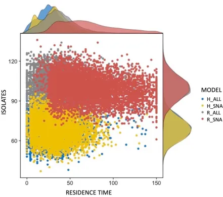
Figure 2. The main environmental outcomes. Comparison for experiment-specific

(21)

21

point found is 0.1. The high ends of the beans are cut to a maximum value of 0.2 for visibility of the distribution. The variability of outcomes across simulations was also greater when all behavioral drivers were included, and the mean level of environmental outcomes was lower with a homophilous network. The models are abbreviated as H_ALL: homophilous network model influenced by all drivers (actor attributes, social network, ecological feedback and cross-scale actors); R_ALL: random network model influenced by all four factors; H_SNA: homophilous network model influenced by social networks and landowner attributes only; and R_SNA: random network model influenced by social networks and actor attributes only. The figure was produced using the beanplot R package (50, 51)

Figure 3. The average temporal variation in the size of protected area during model

simulation. The distribution of residence time (the total duration of land as protected) for the homophily model with all behavioral drivers shows the shortest average duration for

protected areas and no extreme outcomes. The random model excluding external variables produces the most long-term protected areas. The number of isolates plays a role as the fraction of the rural collective that cannot be reached through social networks and was found to be higher in random networks than in survey-based homophilous networks. The figure was produced using the ggpubr R package (50, 52).

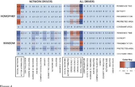
Figure 4. Scenario- and model-specific effect sizes. Behavioral drivers included in decision making by land owners are marked with a black rectangle, and the remaining variables on the y-axis are social network indices. The figure was produced using the gplots R package (50, 53).

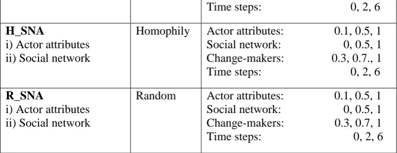
Table 1. Model experiments. In each experiment, the effect of behavioral drivers was tested by systematically changing their influence in decision making. Cross-scale groups include indigenous group (New Zealand Māori iwi), local council representatives and central government representatives. ‘Change-makers’ is the percentage of land owners making a decision during each time step, and ‘time steps’ is the minimum time interval between land use changes. Neither of these is a behavioral driver.

(22)

22

randomization in R_SNA and R_ALL experiments. The full table and descriptions for each social network analysis index can be found in SI tables S3 and S4.

FIGURES

(23)

23

(24)

24

(25)

25 Figure 4.

TABLES

Table 1.

EXPERIMENT AND BEHAVIORAL FACTOR TYPES

NETWORK MODEL

PARAMETER VALUES

H_ALL

i) Actor attributes ii) Social network iii) Cross-scale groups iv) Ecological feedback

Homophily Actor attributes: 0.1, 0.5, 1 Social network: 0, 0.5, 1 Cross-scale groups

- Indigenous: 0, 0.5, 1 - Council: 0, 0.5, 1 - Central gov.: 0, 0.5, 1 Ecological feedback: 0, 0.5, 1 Change-makers: 0.3, 0.7, 1 Time steps: 0, 2, 6

R_ALL

i) Actor attributes ii) Social network iii) Cross-scale groups iv) Ecological feedback

Random Actor attributes: 0.1, 0.5, 1 Social network: 0, 0.5, 1 Cross-scale groups

(26)

26

Time steps: 0, 2, 6

H_SNA

i) Actor attributes ii) Social network

Homophily Actor attributes: 0.1, 0.5, 1 Social network: 0, 0.5, 1 Change-makers: 0.3, 0.7., 1 Time steps: 0, 2, 6

R_SNA

i) Actor attributes ii) Social network

Random Actor attributes: 0.1, 0.5, 1 Social network: 0, 0.5, 1 Change-makers: 0.3, 0.7, 1 Time steps: 0, 2, 6

Table 2. SOCIAL NETWORK INDEX HOMOPHILY NETWORK RANDOM NETWORK

Network size 91.000

142.726 217.000

74.000 139.117 212.000

Bridging actors 26

46.272 70.000

8.000 30.565 60.000

Isolates 37.000

69.262 101.000

61.000 99.657 136.000

Compartmentalization 0.210

0.677 0.911 0.791 0.934 0.974 Average weighted indegree without isolates 0.523 0.723 0.979 0.642 0.918 1.225

Density 0.002

(27)

27

Supplementary Information for:

Effects of multiple behavioral drivers on collective

conservation outcomes

Yletyinen, J.*, Perry, G., Brown, P., Pech, R., Tylianakis, J.M. * Corresponding author: [email protected]

This PDF file includes:

Supplementary text: Network questions

Figure S1a-d. Baseline protected and covenanted area Figure S2. Land owners’ homophily network

Table S1. Survey - based actor attributes and landscape variables Table S2. Environmental outcome variables

Table S3 Structural social network indicators: definitions

Table S4 Structural social network indicators for homophily and random networks

Tables S5a-d. Logistic regression results for actor attributes

Supplementary Materials Appendix A: Overview, design concepts and details (ODD) protocol for Land owner model

Table S5 Model input data: actor attributes Table S6. Model input data: homophily matrix

(28)

28

Supplementary Information Text:

Network questions in the Rural Decision-Makers 2015 Survey

This section describes how the Rural Decision-Makers 2015 survey data (1) were converted to a social network structure. In the social network including only land owners, each node is an individual land owner, and each link represents influence mediated by conversations about environmental issues. First, land owners were asked "Did you regularly meet with individual people from the following groups to discuss environmental performance of your farm

business over the past 12 months?" If a land owner chose "Farmers in your industry" or "Farmers in different industries", they received two additional questions on the number and influence of connections they have to other land owners. The in-degree (number of incoming links) is based on the land owners reply to the question: "With approximately how many individuals from each of the following groups did the trust board regularly meet to discuss environmental performance of the farm business during the past 12 months?". Then, the land owners evaluated the influence ("How influential is advice about environmental performance from these individuals?") on four-categorical scale: not at all influential, slightly influential, moderately influential, extremely influential. The answers were quantified and standardized to numeric link weights (0, 0.33, 0.66, 1). If a land owner replied "Not at all influential", the link weight becomes zero and the land owner’s in-links to other land owners are removed from the network.

(29)

29

Fig.S1a-d.Relationship between baseline habitat and environmental outcomes. Due to diffusion processes (ecological feedback, social network influence), the extent of protected area in the beginning of model simulation affects the extent of protected area and covenanted area in the end of model simulation. (a) shows the relationship between the extent of

(30)

30

(31)

31

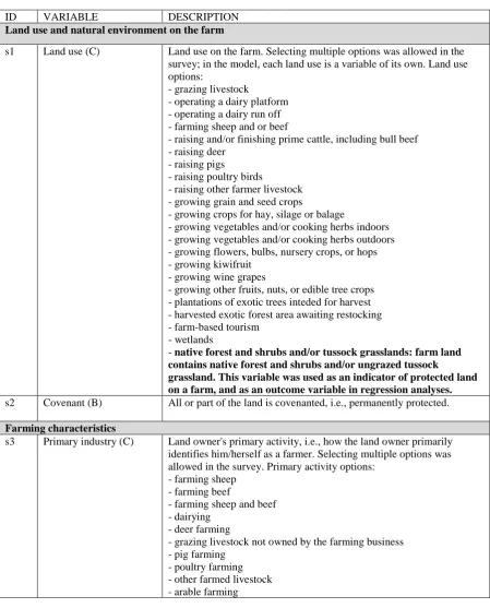
Table S1.Survey-based actor attributes and additional landscape variables included in the model. Prefix 's' in front of the ID number indicates Rural Decision-Makers survey-based variables, whereas variables calculated in the model can be found in Table S2 (prefix 'm'). In the Variable column, a letter indicates the reply options for each survey question: (B) binary (yes/no) reply, (C) categorical reply, (N) a value reported by the land owner. We assume any additional variables to be constant across the land owners throughout the modelled time period. These variables may include economic (e.g., market forces), political (e.g., policies that increase the productivity of the land and make setting aside land for conservation a greater loss) and institutional factors (e.g., attitudes on the public having right to recreational natural spaces).

ID VARIABLE DESCRIPTION

Land use and natural environment on the farm

s1 Land use (C) Land use on the farm. Selecting multiple options was allowed in the survey; in the model, each land use is a variable of its own. Land use options:

- grazing livestock

- operating a dairy platform - operating a dairy run off - farming sheep and or beef

- raising and/or finishing prime cattle, including bull beef - raising deer

- raising pigs

- raising poultry birds

- raising other farmer livestock - growing grain and seed crops

- growing crops for hay, silage or balage

- growing vegetables and/or cooking herbs indoors - growing vegetables and/or cooking herbs outdoors - growing flowers, bulbs, nursery crops, or hops - growing kiwifruit

- growing wine grapes

- growing other fruits, nuts, or edible tree crops - plantations of exotic trees inteded for harvest - harvested exotic forest area awaiting restocking - farm-based tourism

- wetlands

- native forest and shrubs and/or tussock grasslands: farm land

contains native forest and shrubs and/or ungrazed tussock

grassland. This variable was used as an indicator of protected land on a farm, and as an outcome variable in regression analyses. s2 Covenant (B) All or part of the land is covenanted, i.e., permanently protected.

Farming characteristics

s3 Primary industry (C) Land owner's primary activity, i.e., how the land owner primarily identifies him/herself as a farmer. Selecting multiple options was allowed in the survey. Primary activity options:

- farming sheep - farming beef

- farming sheep and beef - dairying

- deer farming

- grazing livestock not owned by the farming business - pig farming

(32)

32

- vegetable production

- growing flowers, bulbs, nursery crops, or hops - kiwifruit production

- wine grape production

- growing fruits, nuts, or edible tree crops - exotic forestry

- farm-based tourism

- native forest and shrubs and/or tussock grassland - other

s4 Ownership (C) Ownership of the land: myself (land owner) / another individual / family partnership / family trust / family company / Māori trust or inc. / corporate owned / equity partnership / family company

s5 Live on farm (C) The land owner lives on the farm: year-round / part of the year / not at all.

s6 Area (N) The total area of the farm in hectares. This variable addresses the largest land parcel of the farm, even if the farm includes additional blocks.

Personal values

s7 Private conservation (C) Private land owners should protect habitat for native plants and animals on private land: strongly disagree / middle / strongly agree.

s8 Public conservation (C) The New Zealand Department of Conservation should protect habitat for native plants and animals on public land: strongly disagree / middle / strongly agree.

s9 Covenant barriers (C) The reasons why land owner has not joined a covenant: don't have suitable land / fear of losing property rights / too much regulations. In the model, each reason is a variable of its own.

Social networks

s10 Indegree (C, N) The number of connections a land owner has to other land owners and to each cross-scale actor group. This variable consists of two parts: i) whether the land owner has regularly met to discuss environmental performance of the farm with representatives from the following actor groups (C); and ii) with approximately how many representatives of each group they have met regularly (N). Indegree for any of the

stakeholder subgroups can be zero if a land owner has no connections to that group. The model includes following network actors:

- regional councils, district councils - central government

- iwi, i.e. largest social units of māori in New Zealand, often translated to “tribe” in English. In this study, we call iwi “indigenous groups”. - farmers in the same industry as land owner

- farmers in different industries than land owner

s11 Social influence (C) Land owner's estimation of how much influence his/her social

(33)

33

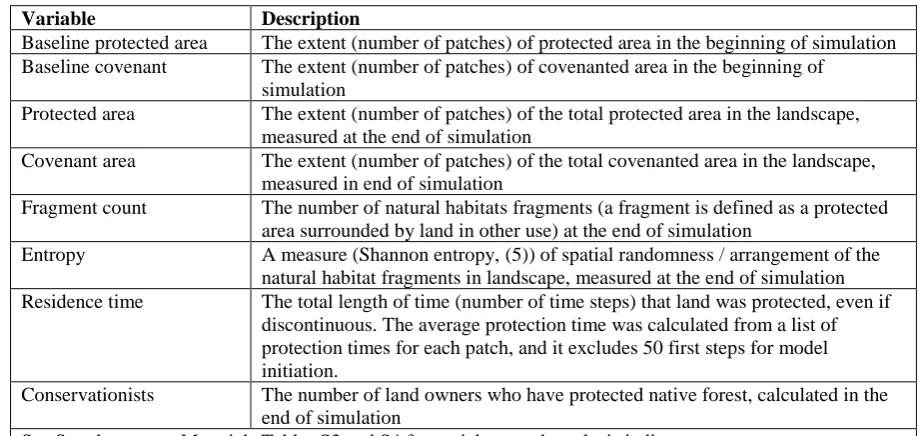
Table S2. State variables included in the study.

Variable Description

Baseline protected area The extent (number of patches) of protected area in the beginning of simulation Baseline covenant The extent (number of patches) of covenanted area in the beginning of

simulation

Protected area The extent (number of patches) of the total protected area in the landscape, measured at the end of simulation

Covenant area The extent (number of patches) of the total covenanted area in the landscape, measured in end of simulation

Fragment count The number of natural habitats fragments (a fragment is defined as a protected area surrounded by land in other use) at the end of simulation

Entropy A measure (Shannon entropy, (5)) of spatial randomness / arrangement of the natural habitat fragments in landscape, measured at the end of simulation Residence time The total length of time (number of time steps) that land was protected, even if

discontinuous. The average protection time was calculated from a list of protection times for each patch, and it excludes 50 first steps for model initiation.

Conservationists The number of land owners who have protected native forest, calculated in the end of simulation

(34)

34

Table S3. Structural social network indices. The indicators included in the

study were chosen based on influence on collective action or environmental management described in previous studies. Due to the high number of isolates in our networks, some indices were calculated with and without isolates.

SOCIAL NETWORK INDICES

INDEX RELEVANCE

Mean path length:the average of shortest paths between all actor (node) pairs (6)

A short mean path indicates that everyone in a network is fairly 'close' to each other, and actors can thus reach each other through a small number of intermediate actors (cohesive network) (6).

Density: the ratio between the actual number of links in a network and the number of possible links (6)

Density affects collective action as increased possibilities for communication (influence), exposure to new ideas and knowledge (7). However, very high density may hinder efficiency of collective action, or lead to homogenization (7). In influence network, short mean path and density would thus lead to quick spread of attitudes, knowledge and behaviour.

Centrality: how central the network's most central actor is in relation to how central all the other actors are (8)

While density and mean path describe the overall cohesion of a network, centralization describes the extent to which this cohesion is organized around particular actor(s) (7). High degree of

centralization may have a positive effect on collective action as a central actor can prioritize certain action, and even coordinate the action, but it also indicates asymmetric influence relations (7). Hence, a highly centralized network would indicate a presence of central actors who are in key position to influence a large proportion of the land owner collective.

Compartmentalization: a presence

of subgroups in which actors are joined together in tightly connected groups, between which there are fewer connections (9)

The low density of links between compartments may have negative effects on the collective action (see Density), and may lead to "them and us" attitudes, but high density inside compartments may lead to developing specialized knowledge (7). In the case of homophilic influence network, compartmentalization indicates subgroups of like-minded people with fewer connections (that would allow spread of attitudes and behaviour) to people less similar to them.

Bridging links: links connecting different actor subgroups. Here, we measure bridging links as number of cut points (articulation points): actors whose removal increases the number of connected components in a network by forming two or more separate subgroups between which there are no connections(6).

By connecting network subgroups (potentially compartments), bridging links provide actors in subgroups access to external knowledge and resources. Thus, high number of bridges enable or support collective action among different groups of actors. In this study, we calculated number of cut-points (i.e. actors who connect subgroups/network components. Removal of cut-point actors leads to a network subgroup breaking into two with no communication in between) to indicate number of bridgers.

Isolates: non-connected actors Actors who do not participate in local network because they do not

have links to other actors (based on the network boundary setting). In our study, actors who had not had frequent, influential discussion about environmental performance of the farm. Our ‘Isolates’ network index shows number of isolates.

Average weighted degree: the

average number of connections that actors in a network have, including the link weights.

(35)

35

Table S4. Structural social network indicators for homophily and random networks. The bold value is the mean (for which standard error (SD) is calculated), value above it the minimum value, and below it the maximum value for all simulations. Due to the high number of isolates in our networks, we have calculated some indices with and without isolates. Network size is the number of links in the network. Erdős–Rényi randomization was based on the average density of homophily networks, and should thus be similar for homophily and random networks.

SOCIAL NETWORK INDEX HOMOPHILY NETWORK HOMOPHILY SD RANDOM NETWORK RANDOM SD

Mean path length 1.224

2.210

6.232 0.569

1.211

2.528

8.496 0.808

Network size 91.000

142.726

217.000 16.154

74.000

139.117

212.000 16.760

Number of cut points 26

46.272

70.000 6.175

8.000

30.565

60.000 6.522

Centralization 0.007

0.015

0.030 0.003

0.006

0.016

0.032 0.004 Centralization

without isolates

0.008

0.021

0.050 0.005

0.006

0.025

0.067 0.007 Average weighted indegree 0.289

0.473

0.729 0.057

0.205

0.461

0.704 0.060 Average weighted indegree

without isolates

0.523

0.723

0.979 0.060

0.642

0.918

1.225 0.068 Compartmentalization 0.210

0.677

0.911 0.095

0.791

0.934

0.974 0.019

Density 0.002

0.004

0.005 0.000

0.002

0.003

0.005 0.000 Density without isolates 0.006

0.008

0.012 0.001

0.010

0.014

0.021 0.001

Isolates 37.000

69.262

101.000 8.689

61.000

99.657

(36)

36

Tables S5a-d. Stepwise logistic regression analyses with forward selection were used to examine which variables could influence land owner’s probability to protect native habitat for biodiversity, and thus, be used as actor attributes. Tables S5a shows maximal models with variable “farm land contains native forest and shrubs and/or ungrazed tussock grassland”

(Table S1 variable s1), and Table S5c maximal model with variable “All or part of the land is covenanted” (Table S1 variable s2) as dependent variables. S5b and S5c present the results, respectively. The results include only land use variables. This is partly because both our dependent variables were essentially describing land use. Further, it is likely that land

owners’ values, ownership and choices required by the primary industry are already reflected in land use. Collinearity was detected only for land use variables. Significance codes for p-values: ***: < 0.001, ** < 0.01, * < 0.05, . < 0.1.

Table S5a. ID

Variable Estimate

Std. Error

z

value Pr(>|z|) (Intercept)

-1.95E+00 2.11E+00

-0.926 0.354311 s7 Private land owners should protect habitat for

native plants and animals on private land: 7 -5.31E-01 4.27E-01

-1.655 0.097961 . s7 Private land owners should protect habitat for

native plants and animals on private land: 10 -9.22E-01 4.80E-01 -1.92 0.054872 . s8 The Department of Conservation should

protect habitat for native plants and animals on public land: 1

-1.51E+01 3.96E+03

-0.004 0.996959 s8 The Department of Conservation should

-1.52E+01 1.94E+03

-2.95E+01 1.95E+03

protect habitat for native plants and animals

on public land: 4 -5.26E-01 2.37E+00

on public land: 5 3.57E-01 2.11E+00 0.169 0.866028 s8 The Department of Conservation should

on public land: 6 -9.83E-01 2.07E+00

on public land: 7 -1.38E-01 2.04E+00

on public land: 8 -4.89E-01 2.03E+00

on public land: 9 5.75E-02 2.04E+00 0.028 0.977491 s8 The Department of Conservation should

(37)

37 s4

Land ownership: myself

-1.35E+00 1.14E+00

-1.176 0.239723 s4

Land ownership: another individual -2.04E-01 4.18E-01

-0.487 0.626112 s4

Land ownership: family partnership -1.66E-01 4.33E-01

-0.384 0.701343 s4 _{Land ownership: family trust} _{2.64E+00 1.68E+00} _1.568 _0.116814 s4

Land ownership: family company

-1.71E+01 1.14E+03

-0.015 0.988042 s4 _{Land ownership: māori trust / inc.} _3.98E-01 _6.45E-01 _0.618 _0.536722 s4 _{Land ownership: corporate owned} _6.35E-01 _4.70E-01 _1.35 _0.177038

s6 _Area _8.61E-05 _1.31E-04 _0.658 _0.510582

s3

Primary industry: grazing livestock, not own -9.33E-01 6.90E-01

-1.353 0.175908 s3

Primary industry: farming sheep -4.61E-01 6.57E-01

-0.701 0.483603 s3

Primary industry: farming beef -5.64E-01 6.57E-01

-0.857 0.391223 s3 _{Primary industry: dairying} _{5.22E-01 1.25E+00} _0.418 _0.675597 s3 _{Primary industry: deer farming} _{1.06E-01 1.12E+00} _0.095 _0.924602 s3

Primary industry: pig farming -1.36E-01 1.54E+00

-0.089 0.929438 s3

Primary industry: poultry farming

-1.49E+01 1.96E+03

-0.008 0.993943 s3

Primary industry: other farmed livestock

-2.58E+00 1.42E+00

-1.816 0.069396 . s3

Primary industry: arable farming -7.95E-02 1.07E+00

-0.074 0.940855 s3 _{Primary industry: vegetable production} _{3.43E-01 1.25E+00} _0.275 _0.782999 s3

Primary industry: kiwifruit production -2.76E-01 2.54E+00

-0.109 0.913228 s3

Primary industry: wine grape production

-3.23E+01 1.73E+03

-0.019 0.985098 s3 Primary industry: growing fruits, nuts, edible

tree crops 3.94E-01 9.99E-01 0.394 0.693245 s3

Primary industry: exotic forestry

-1.39E+00 8.45E-01

-1.642 0.100517 s3 _{Primary industry: farm-based tourism} _{1.06E+00 1.25E+00} _0.85 _0.39556 s3 _{Primary industry: other} _{1.56E+01 3.96E+03} _0.004 _0.996853 s3 _{Land use: cattle} _2.42E-01 _2.95E-01 _0.822 _0.411148 s1

Land use: dairy platform

-1.03E+00 1.07E+00

-0.962 0.33589 s1

Land use: dairy runoff -1.64E-01 5.71E-01

-0.287 0.773911 s1

Land use: deer -5.51E-01 7.09E-01

-0.777 0.437357 s1

Land use: flowers -1.29E-01 1.27E+00

-0.102 0.918701 s1 _{Land use: forestry} _2.31E+00 _3.36E-01 _6.879 _{6.05E-12 ***} s1 _{Land use: forestry harvested} _5.46E-01 _8.39E-01 _0.651 _0.515249 s1

Land use: fruit -6.23E-01 6.74E-01

-0.925 0.354869 s1

Land use: grain seeds