A Machine Learning Approach for Air Quality
Prediction: Model Regularization and Optimization
Dixian Zhu1*, Changjie Cai2, Tianbao Yang3and Xun Zhou4
1 Department of Computer Science, University of Iowa; [email protected]
2 Department of Occupational and Environmental Health, University of Iowa; [email protected]
3 Department of Computer Science, University of Iowa; [email protected]
4 Department of Management Sciences, University of Iowa; [email protected]
* Correspondence: [email protected]
Abstract: In this paper, we tackle air quality forecasting by using machine learning approaches to 1
predict the hourly concentration of air pollutants (e.g., Ozone, PM2.5and Sulfur Dioxide). Machine 2
learning, as one of the most popular techniques, is able to efficiently train a model on big data by using 3
large-scale optimization algorithms. Although there exists some works applying machine learning 4
to air quality prediction, most of the prior studies are restricted to small scale data and simply train 5
standard regression models (linear or non-linear) to predict the hourly air pollution concentration. 6
In this work, we propose refined models to predict the hourly air pollution concentration based 7
on meteorological data of previous days by formulating the prediction of 24 hours as a multi-task 8
learning problem. It enables us to select a good model with different regularization techniques. We 9
propose a useful regularization by enforcing the prediction models of consecutive hours to be close 10
to each other, and compare with several typical regularizations for multi-task learning including 11
standard Frobenius norm regularization, nuclear norm regularization,`2,1norm regularization. Our 12
experiments show the proposed formulations and regularization achieve better performance than 13
existing standard regression models and existing regularizations. 14
Keywords:air pollutant prediction; multi-task learning; regularization; analytical solution 15
1. Introduction 16
Adverse health impacts from exposure to outdoor air pollutants are complicated functions of 17
pollutant composition and concentration [1]. Major outdoor air pollutants in cities include ozone 18
(O3), particle matters (PMs), sulfur dioxide (SO2), carbon monoxide (CO), nitrogen oxides (NOx), 19
volatile organic compounds (VOCs), pesticides, and metals among others [2,3]. Increased mortality 20
and morbidity rates have been found in association with increased air pollutant (such as O3, PMs and 21
SO2) concentrations [3–5]. According to the report from the American Lung Association [6], 10 part 22
per billion (ppb) increase in O3mixing ratio might cause over 3,700 premature deaths annually in the 23
United States (U.S.). Chicago, like many other megacities in U.S, has struggled with air pollution due to 24
the industrialization and urbanization. Although O3precursor (such as VOCs, NOx, and CO) emissions 25
have significantly decreased since the late 1970’s, O3in Chicago has not been in compliance with 26
standards set by the Environmental Protection Agency (EPA) to protect public health [7]. Particle size is 27
critical in determining the particle deposition location in human respiratory system [8]. PM2.5, referring 28
to particles diameter smaller than or equal to 2.5 micrometer (µm), has been increasingly concerned 29
since they can deposit into the lung gas-exchange region-Alveoli [9]. The U.S. EPA revised the annual 30
standard of PM2.5by lowering the concentration to 12 microgram per cubic meter (µg/m3) to provide 31
improved protection against health effects associated with long- and short-term exposures [10]. SO2, 32
as an important precursor of new particle formation and particle growth, has also been found to be 33
association with respiratory diseases in many countries [11–15]. Therefore, we selected O3, PM2.5and 34
SO2for testing in this study. 35
Meteorological conditions, including regional and synoptic meteorology, are critical in 36
determining the air pollutant concentrations [16–21]. According to the study from Holloway et 37
al. [22], the O3concentration over Chicago was found to be the most sensitive to air temperature, 38
wind speed and direction, relative humidity, incoming solar radiation, and cloud cover. For example, 39
the lower ambient temperature and incoming solar radiation slows down photochemical reactions 40
and leads to less secondary air pollutants, such as O3 [23]. Increasing wind speed could either 41
increase or decrease the air pollutant concentrations. For instance, when the wind speed was 42
low (week dispersion/ventilation), the pollutants associated with traffic were found at highest 43
concentrations [24,25]. However, the strong wind speed might form the dust storms by blowing 44
up the particles on the ground [26]. High humidity is usually associated with high concentrations of 45
certain air pollutants (such as PMs, CO and SO2), but with low concentrations of other air pollutants 46
(such as NO2and O3) due to various formation and removal mechanisms [25]. In addition, high 47
humidity can be an indicator of precipitation events, which results in strong wet deposition leading to 48
low concentrations of air pollutants [27]. Since various particle compositions and their interactions 49
with light were found as the most important factors in attenuating visibility [28–30], low visibility could 50
be an indicator of high PM concentrations. Cloud can scatter and absorb the solar radiation, which 51
is significant for the formation of some air pollutants (e.g., O3) [23,31]. Therefore, these important 52
meteorological variables were selected to predict air pollutant concentrations in this study. 53
Statistical models have been applied for air pollution prediction based on meteorological data [33, 54
34,36]. However, existing studies on statistical modeling are mostly restricted to simply utilizing 55
standard classification or regression models, which have neglected the nature of the problem itself or 56
ignore the correlation between each hour’s model. On the other hand, machine learning approaches 57
have been developed for over 60 years and have achieved tremendous success in many areas [32, 58
42–46]. There exist various new tools and techniques invented in machine learning community, 59
which allow for more refined modeling for a specific problem. In particular, model regularization 60
is a fundamental technique for improving the generalization performance of a predictive model. 61
Accordingly, many efficient optimization algorithms have been developed for solving various machine 62
learning formulations with different regularizations. 63
In this study, we focus on refined modeling for predicting hourly air pollutant concentration 64
based on historical metrological data and air pollution data. A striking difference between this work 65
and the previous works is that we emphasize on how to regularize the model in order to improve 66
its generalization performance, and how to learn a complex regularized model from big data with 67
advanced optimization algorithms. We have collected 10 years of meteorological and air pollution 68
data in the Chicago area. The meteorological data is from MesoWest [53] and the air pollutant data 69
is from the EPA [51,52]. From their databases, we fetch consecutive hourly measurements of various 70
meteorological variables and pollutants reported by two air quality monitoring stations and two 71
air pollutant monitoring sites in the Chicago area. Each record of hourly measurements includes: 72
meteorological variables like solar radiation, wind direction and speed, temperature, atmospheric 73
pressure; and air pollutants include PM2.5, O3, SO2. We use two methods for model regularization: 74
(i) explicitly control the number of parameters in the model; (ii) explicitly enforce certain structure 75
in the model parameters. For controlling the number of parameters in the model, we compare three 76
different model formulations which can be considered in a unified multi-task learning framework 77
with a diagonal or full matrix model. For enforcing the model matrix into a certain structure, we will 78
consider the relationship between prediction models of different hours and compare three different 79
regularizations with standard Frobenius norm regularization. The experimental results show that 80
the model with the intermediate size and the proposed regularization that enforces the prediction 81
models of two consecutive hours to be close achieve the best results and are much better than standard 82
regression models. We also develop efficient optimization algorithms for solving different formulations 83
The rest of the paper is organized as follows. In section 2, we discuss related work. In section 85
3, we describe data collection and preprocessing. In section 4, we described the proposed solutions, 86
including formulations, regularizations and optimizations. In section 5, we present the experimental 87
studies and the results. In section 6, we give conclusions, and indicate future work. 88
2. Related Work 89
A large number of previous work has been done to apply machine learning algorithms onto air 90
quality predictions. Some researchers aimed to predict targets into discretized levels. Kalapanidas et 91
al. [34] elaborated effects on air pollution only from meteorological features such as temperature, wind, 92
precipitation, solar radiation, and humidity, and classified air pollution into different levels (low, med, 93
high, alarm) by using a lazy learning approach, Case Based Reasoning (CBR) system. Athanasiadis et 94
al. [35] employedσ-fuzzy lattice neurocomputing classifier to predict and categorize O3 concentration 95
into 3 levels (low, mid, and high) based on meteorological features and other pollutants like SO2, 96
NO, NO2and so on. Kunwar et al. [36] utilized principle component analysis (PCA) and ensemble 97
learning models to predict categorized air quality index (AQI) and combined air quality index (CAQI). 98
However, the process of converting regression tasks to classification tasks is problematic, as it ignores 99
the magnitude of the numeric data and consequently is inaccurate. 100
Other researchers worked on predicting concentrations of pollutants. Corani [37] worked on 101
training neural network models to predict hourly O3and PM10 concentration based on data from the 102
previous day. Performances of Feed Forward Neural Network (FFNN) and Pruned Neural Network 103
(PNN) were mainly compared. More efforts have been made on FFNN, Fu et al. [38] applied a rolling 104
mechanism and gray model to improve traditional FFNN models. Jiang et al. [39] explored multiple 105
models (physical & chemical model, regression model, multiple layer perceptron) on the air pollutant 106
prediction task and their result shows statistical models are competitive to the classical physical & 107
chemical models. Ni, X. Y. et al. [40] compared multiple statistical models based on PM2.5data around 108
Beijing, which implies linear regression models sometimes can be better than the other models. 109
Multi-task Learning (MTL) focuses on learning multiple tasks that have commonalities 110
together [41], which can improve the efficiency and accuracy of the models. It has achieved 111
tremendous successes in many fields such as: natural language processing [42], image recognition [43], 112
bioinformatics [44,45], marketing prediction [46], etc. A variety of regularizations can be utilized to 113
enhance the commonalities of the tasks including`2,1-norm [47], nuclear-norm [48], spectral norm [49]], 114
Frobenius norm [50], etc. However, most of former machine learning works on air pollutant prediction 115
don’t consider the similarities between the models and only focus on improving model performance 116
for a single task. 117
Therefore, we decide to use meteorological and pollutant data to do prediction for hourly 118
concentration based on linear models. In this work, we focus on three different prediction model 119
formulations and using MTL framework with different regularizations. To the best of our knowledge, 120
this is the first work that utilizes MTL on air pollutant prediction task. We exploit analytical approaches 121
and optimization techniques to obtain the optimal solutions. The model evaluation metric is rooted 122
mean squared error (RMSE). 123
3. Data Collection and Preprocessing 124
3.1. Data Collection 125
We collected air pollutant data from two air quality monitoring sites, and meteorological 126
data from two weather stations from 2006 to 2015 (summarized in Table 1). The air pollutants 127
include the concentrations of O3, PM2.5 and SO2 in this study. We downloaded the air pollutant 128
data from the U.S. Environmental Protection Agency’s (U.S. EPA) Air Quality System (AQS) 129
database (https://www.epa.gov/outdoor-air-quality-data), which has been widely used for model 130
Table 1.Summary of measurement sites and observed variables
Measurement sites Variables
Alsip Village (AV) O3and PM2.5
Lemont Village (LV) O3and SO2
Lansing Municipal Airport (LMA)
temperature, relative humidity, wind speed, wind direction, wind gust, precipitation accumulation, visibility, dew point, wind cardinal direction, pressure, and weather condition
Lewis University (LU) The same as LMA site
concentrations including air temperature, relative humidity, wind speed, wind direction, wind gust, 132
precipitation accumulation, visibility, dew point, wind cardinal direction, pressure, and weather 133
condition. We downloaded the meteorological data from MesoWest (http://mesowest.utah.edu/), a 134
project within the Department of Meteorology at the University of Utah, which has been aggregating 135
meteorological data since 2002 [53]. 136
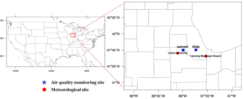
The locations of the two air quality monitoring sites and two weather stations are shown in 137
(Figure1). The Alsip Village (AV) air quality monitoring site is also located in a suburban residential 138
area, which is in south Cook County, Illinois (AQS ID: 17-031-0001; lat/long: 41.670992/-87.732457). 139
The Lemont Village (LV) air quality monitoring site is located in a suburban residential area, which is 140
in southwest Cook County, Illinois (AQS ID: 17-031-1601; lat/long: 41.66812/-87.99057). The weather 141
state situated in Lansing Municipal Airport (LMA) is the closest meteorological site (MesoWest ID: 142
KIGQ; lat/long: 41.54125/-87.52822) to the AV air quality monitoring site. The weather station 143
positioned in Lewis University (LU) is the closest meteorological site (MesoWest ID: KLOT; lat/long: 144
41.60307/-88.10164) to the LV air quality monitoring site. 145
Figure 1.Locations of measurement sites.Blue starsdenote the two air quality monitoring sites.Red
circlesdenote the two meteorological sites.
3.2. Preprocessing 146
We paired the collected meteorological data and air pollutant data based on time to obtain the 147
required data format of applying the machine learning methods. In particular, for each variable we 148
form one value for each hour. However, the original data may contain multiple values or missing 149
values at some hours. To preprocess the data, we calculated the hourly mean value of each numeric 150
variable if there are multiple observed values within an hour, and chose the category with the highest 151
frequency per hour for each categorical variable if there are multiple values. Missing values exist for 152
some variables, which are not tolerable of applying the machine learning methods used in this study. 153
variables and one categorical variable, including wind gust, pressure, altimeter, precipitation, and 155
weather condition. We deleted the days which still have missing values after imputing. We applied 156
dummy coding for two categorical variables, the cardinal wind direction (16 values) and weather 157
condition (31 values). Then, we added weekday and weekend as two boolean features. Finally, 158
we obtained 60 features in total (9 numerical meteorological features + 16 dummy coding for wind 159
direction + 31 dummy coding for weather condition + 2 boolean feature for weekday/weekend + 1 160
numerical feature for pollutant + 1 bias term). We apply normalization for all the features and pollutant 161
targets to make their values fall in[0, 1]. 162
4. Machine Learning Approaches for Air Pollution Prediction 163
In this section, we will describe the proposed approaches for predicting the ambient concentration 164
of air pollutants. 165
4.1. A General Formulation 166
Our goal is to predict the concentration of air pollutants of next day based on the historical 167
meteorological and air pollutant data. In this work we focus on using the former day’s data to 168
predict this day’s hourly based pollutants. In particular, let(xi;yi)denote thei-th training data where
169
yi ∈ R24×1 denotes the concentration of a certain air pollutant at a day andxi = (ui;vi) denotes
170
the observed data in the previous day that include two components, where ‘;’ represents column 171
layout. The first componentui = (ui,1; . . . ;ui,D) ∈ R24·D×1 include all meteorological data of 24
172
hours in the previous day, whereui,j∈R24×1denotes thej-the meteorological feature of 24 hours and
173
Dis the number of meteorological features, and the second componentvi ∈ R24×1include hourly
174
concentration of the same air pollutant in the previous day. The general formulation can be expressed 175
as: 176
min
W
1 n
n
∑
i=1
kf(W,xi)−yik22+ϕ(W) (1)
where W denote the parameters of the model, f(W,xi) denotes the prediction of air pollutant
177
concentration, andϕ(·)denotes a regularization function of the model parametersW. 178
Next, we introduce two levels of model regularization. The first level is to explicitly control the 179
number of model parameters. The second level is to explicitly impose a certain regularization on the 180
model parameter. For the first level, we consider three models that are described below: 181
• Baseline Model. The first model is a baseline model that has been considered in existing studies and has the least number of parameters. In particular, the prediction of the air pollutant concentration is given by
fk(W,xi) = D
∑
j=1
e>kui,j·wj+e>k vi·wD+1+w0, k=1, . . . , 24
whereek∈R24×1is a basis vector with only one at thek-th position and zeros at other positions.
182
w0,w1, . . . ,wD,wD+1∈Rare the model parameters, wherew0is the bias term. Denote byW =
183
(w0,w1, . . . ,wD+1)>for this model. It is notable that this model predicts the hourly concentration 184
based on the same hour historical data in the previous day and hasD+2 parameters. This 185
• Heavy Model. The second model will take all the data in previous day into account when predicting the concentration of every hour in the second day. In particular, for thek-th hour, the prediction is given by
fk(W,xi) = D
∑
j=1
ui,j>wk,j+vi>wk,D+1+wk,0, k=1, . . . , 24
wherewk,j∈R24×1,j=1, . . . ,D+1 andwk,0∈R. For this model, we define:
W =
w1,0 w2,0 . . . w24,0 w1,1 w2,1 . . . w24,1 . . . . w1,D+1 w2,D+1 . . . w24,D+1
Note that each column ofWcorresponds to the prediction model for each hour. There are a total 187
of 24×(24∗(D+1) +1)parameters. It is notable that the baseline model is a special case by 188
enforcing all columns ofWto be the same and eachwk,jhas only one non-zero element in the
189
k-th position. 190
• Light Model. The third model is between the baseline model and the heavy model. It considers the 24 hours pattern of the air pollutant in the previous day and the same hour meteorological data in the previous day to predict the concentration at a particular hour. The prediction is given by
fk(W,xi) = D
∑
j=1
e>kui,j·wk,j+v>i wk,D+1+wk,0, k=1, . . . , 24
wherewk,j ∈R,j=1, . . . ,Dandwk,D+1∈R24×1. For this model, we define:
W =
w1,0 w2,0 . . . w24,0 w1,1 w2,1 . . . w24,1 . . . . w1,D+1 w2,D+1 . . . w24,D+1
It is also notable that each column correspond to the predictive model of one hour, andWhas a 191
total of 24∗(D+1) +24∗24∗1 parameters. 192
4.2. Regularization of Model Parameters 193
In this section, we describe different regularizations for the model parameter matrixWin the 194
heavy and light model. We consider the problem as multi-task learning, where predicting the 195
concentration of air pollutant at one hour is one task. In literature, a number of regularizations have 196
been proposed by considering the relationship between different tasks. We first describe three baseline 197
regularizations in literature and then present the proposed regularization that take the dimension of 198
time into consideration for modeling the relationship between models at different time. 199
• Frobenius norm regularization. Frobenius norm regularization is a generalization of standard Euclidean norm regularization to the matrix case, where
ϕ(W) =λ||W||2F,
whereλ>0 is a regularization parameter. 200
(across different tasks) and the computing the`1norm of the resulting vector. In particular, for W∈Rd×K
kWk2,1 =
d
∑
j=1
kWj,∗k2,
whereWj,∗denotes thej-th row ofW. We will consider aL2,1-norm regularizerϕ(W) =λkWk2,1. 201
• Nuclear norm regularization. Nuclear norm is defined as the sum of singular values of a matrix, 202
which is a standard regularization for enforcing a matrix to have a low rank. The motivation 203
of using a low rank matrix is that models for consecutive hours are highly correlated, which 204
could render the matrixWto be low rank. Denote bykWk∗the nuclear norm of a matrixW, the 205
regularization isϕ(W) =λkWk∗. 206
• Consecutive-Close (CC) Regularization. Finally, we propose a useful regularization for the considered problem that explicitly enforces the predictive models for two consecutive hours to be close to each other. The intuition is that usually the concentration of air pollutants for two consecutive hours are close to each other. Denote byW = (w1, . . . ,wK)and by Cons(W) = [(w1−w2),(w2−w3), ...,(wK−1−wK)]. The consecutive-close regularization is given by
ϕ(W) =λ
K−1
∑
j=1
kwj−wj+1k
p
p (2)
wherep=1 orp=2. 207
4.3. Stochastic Optimization Algorithms for Different Formulations 208
Except that Frobenius norm regularized model (with`2norm consecutive-close regularization 209
or not) has a closed-form solution, we solve the other models via advanced stochastic optimization 210
techniques. DenoteF(W,xi) = [f1(W,xi), ...,f24(W,xi)],Yi = [yi,1, ...,yi,24], and the total number of 211
feature isD. Although the standard stochastic (sub)gradient method [54] can be utilized to solve all the 212
formulations considered in this work, it does not necessary yield the fastest convergence. To address 213
this issue, we will consider advanced stochastic optimization techniques tailored for solving each 214
formuation. 215
4.3.1. Optimizing`2,1-norm Regularized Model 216
We utilize Accelerated Stochastic Subgradient (ASSG) Method [55] with proximal mapping to optimize this model. The algorithm runs in mutliple stages and each stage calls the standard stochastic gradient method with a constant step size. To handle the non-smooth`2,1norm, we use the proximal mapping [56]. The stochastic gradient descent part is:
Wt0=Wt−1−2ηs
∂F(Wt−1,xi)
∂Wt−1
e>(F(Wt−1,xi)−Yi) (3)
whereηsis stage-wised stepsize,iis a sampled index, andeis a vector with all 1 as its elements. Then
a proximal mapping is followed (denote by ˜λ=2ηsλ):
Wt=arg min
W kW−W
0tk2
The above problem can solved exactly. Denotewias column vector forW>,w0ias column vector for
W0>t . Then the solution to (4) can be computed by [47]:
wi =
(1− λ˜
kw0ik2
)w0i, ˜λ>0,kw0ik2>λ˜
0, ˜λ>0,kw0ik2≤λ˜
w0i, ˜λ=0
(5)
The pseudocode of the algorithm is as following: 217
Algorithm 1:ASSG with proximal mapping solving`2,1norm regularized model Input:X,Y,W0,η0,S,T
fors=1, . . . ,Sdo ηs=ηs−1/2 fort=1, . . . ,Tdo
Samplei∈ {1, ...,n}
UpdateWt0using equation (3)
UpdateWtusing equation (4)
end
W0=∑Tt=1W1/WT
end
Output:W0 218
4.3.2. Optimizing Nuclear norm Regularized Model 219
The challenge in solving a nuclear norm reguralized problem of most optimization algorithm 220
lies at computing the full singular value decomposition (SVD) of the inovlved matrixW, which is 221
an expensive operation. To avoid full SVD, SVD-freE CONvex-ConcavE Algorithm Extension to 222
Stochastic Setting (SECONE-S) [57] is employed to solve the problem. The algorithm solves the 223
following min-max problem: 224
min
W∈RD×K
max
U∈RD×K
1 n
n
∑
i=1
kF(W,xi)−Yik22+λtr(U>W)−ρ[kUk2−1]+.
Then Stochastic gradient descent and ascent are used to updateWandUat each iteration:
Wt=Wt−1−ηt−1(2
∂F(Wt−1,xi)
∂Wt−1 e
>
(F(Wt−1,xi)−Yi) +λUt−1)
Ut=Ut−1+τt−1(λWt−1−ρ∂[kUt−1k2−1]+),
(6)
whereρ≥ kYk2F, and∂[kUtk2−1]+can be computed byu1v>11[σ1>1]with(u1,v1)being the top left 225
and right singular vectors ofUtandσ1being the top singular value. The pseudocode for the algorithm 226
is as following: 227
Algorithm 2:SECONE-S solving Nuclear norm Regularized Model Input:X,Y,T,η0,τ0
fort=1, . . . ,Tdo Samplei∈ {1, ...,n}
UpdateWtandUtusing equation (6).
ηt=η0/
√
t,τt=τ0/
√
t end
Output: ˆWT=∑t=T 1Wt/T
4.3.3. Optimizing Consecutive-Close Regularized Model 229
The challenge of tackling the proposed consecutive-close regularization lies that the standard 230
proximal mapping cannot be computed efficiently. We address this challenge by using alternating 231
directon method of multipliers. We utilize a recently proposed locally adaptive stochastic alternating 232
direction method of multipliers (LA-SADMM) [58] to solve consecutive-close regularized model. 233
Below, we discuss the updates for the choice ofp=1 (i.e., using the`1norm) in (2). The updates for 234
the choice ofp=2 can be derived similarly. 235
The objective function can be written as:
min
W∈RD×K
1 n
n
∑
i=1
kF(W,xi)−Yik22+λkWEk1,1,
whereE= (eˆ1, ..., ˆek−1), ˆei = (0, ..., 1,−1, ..., 0)T, i =1, ...,k−1, wherei-th element is 1 andi+1-th
element is−1. Therefore,Cons(W) =WE. A dummy variableU=WEis introduced to decouple the last term from the first term and a Lagrangian function is formed as follows:
L(W,U,Λ) = 1
n
n
∑
i=1
kF(W,xi)−Yik22+λkUk1,1−tr(Λ>(WE−U)) +
β
2kWE−Uk 2
F, (7)
whereΛis the Lagrangian multiplier andβis the penalty parameter. 236
Then it can be solved by optimizing each variable alternatively. The update rules for stochatic ADMM (SADMM):
Wτ =arg min
W∈RD×KL(W,Uτ−1,Λτ−1) =arg minW∈
RD×K
˜
F(Wτ−1,xi) +tr{
∂F˜(Wτ−1,xi)
∂W
>
(W−Wτ−1)}
+β
2kWE−Uτ−1− 1
βΛ
T
τ−1k 2
F+
kW−Wτ−1k2F
ητ−1 Uτ =arg min
U∈RD×KL(Wτ,U,Λτ−1) =arg minU∈
RD×K
γkUk1,1+
β
2kWτE−U− 1
βΛ
T
τ−1k 2
F
Λτ=Λτ−1−β(WτE−Uτ)
T,
(8)
where ˜F(Wτ−1,xi) =kF(Wτ−1,xi)−Yik22. 237
LA-SADMM solve the problem more efficiently by doing stage wised penalty increasing. The 238
pseudocode for the algorithm is as following: 239
Algorithm 3:LA-SADMM solving Consecutive-Close Regularized problem with`1norm Input:X,Y,W0,U0,Λ0,β1,η1,S,T
fors=1, . . . ,Sdo forτ=1, . . . ,Tdo
Samplei∈ {1, ...,n}
UpdateWτ,Uτ,Λτusing equation (8). end
WT =∑Tτ=1Wτ/T
W0=WT,U0=UT,Λ0=ΛT
βs+1=2βs,ηs+1=ηs/2
end
Output:WT
5. Experiments 241
We use the names of the paired air quality monitoring sites and two weather stations to denote 242
the two datasets, i.e., LU-LV and LMA-AV. The LU-LV contains the data to predicting the concentration 243
of two air pollutants, i.e., O3and SO2. The LMA-AV contains the data to predicting the concentration 244
of two air pollutants, i.e., O3and PM2.5. 245
We compare 11 different models that are learned with different combinations of model 246
formulations and regularizations. The 11 models are: 247
• Baseline: the baseline model with a standard Frobinus norm regularization. 248
• Heavy-F: the heavy model with a standard Frobinus norm regularization. 249
• Light-F: the heavy model with a standard Frobinus norm regularization. 250
• Heavy-L2,1: the heavy model with aL2,1-norm regularization. 251
• Heavy-Nuclear: the heavy model with a nuclear-norm regularization. 252
• Heavy-CCL2: the heavy model with the consecutive-close regularization using`2norm. 253
• Heavy-CCL1: the heavy model with the consecutive-close regularization using`1norm. 254
• Light-L2,1: the light model with aL2,1-norm regularization. 255
• Light-Nuclear: the light model with a nuclear-norm regularization. 256
• Light CCL2: the light model with the consecutive-close regularization using`2norm. 257
• Light CCL1: the light model with the consecutive-close regularization using`1norm. 258
We divide each dataset into two parts: training data and testing data. Each model is trained on 259
the training data with a proper regularization parameter selected based cross-validation. Each trained 260
model is evaluated on the testing data. The splitting of data is done by dividing all days into a number 261
of chunks of 11 consecutive days, where the first 8 days are used for training and the next 3 days are 262
used for testing. We use the root mean square error (RMSE) as the evaluation metric. 263
0 5 10 15
F L2,1 Nuclear CCL2 CCL1
Im
pr
ov
in
g
Pe
rc
en
ta
ge
(%
)
LU-LV: O3
Heavy Light
(a) grouped by regularizations
0 5 10 15
Heavy Light
Im
pr
ov
in
g
Pe
rc
en
ta
ge
(%
)
LU-LV: O3
F L2,1 Nuclear CCL2 CCL1
(b) grouped by model formulations
-1 0 1 2 3
F L2,1 Nuclear CCL2 CCL1
Im
pr
ov
in
g
Pe
rc
en
ta
ge
(%
)
LU-LV: SO2
Heavy Light
(c) grouped by regularizations
-1 0 1 2 3
Heavy Light
Im
pr
ov
in
g
Pe
rc
en
ta
ge
(%
)
LU-LV: SO2
F L2,1 Nuclear CCL2 CCL1
(d) grouped by model formulations
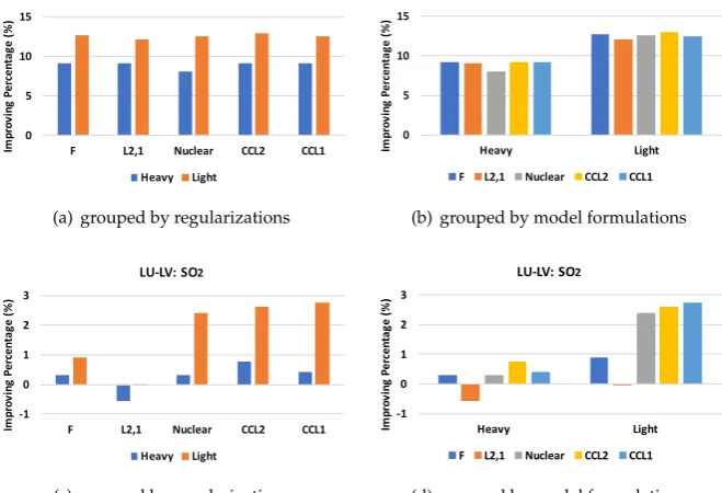
Figure 2.Improvement of Different Methods over the Baseline Method on LU-LV dataset.
We first report the improvement of each method over the Baseline method. The improvement 264
is measured by positive or negative percentage over the performance of the Baseline method, i.e., 265
(RMSE of compared method - RMSE of the Baseline method)*100/RMSE of the Baseline Method. The 266
0 5 10 15
F L2,1 Nuclear CCL2 CCL1
Im
pr
ov
in
g
Pe
rc
en
ta
ge
(%
)
LMA-AV: O3
Heavy Light
(a) grouped by regularizations
0 5 10 15
Heavy Light
Im
pr
ov
in
g
Pe
rc
en
ta
ge
(%
)
LMA-AV: O3
F L2,1 Nuclear CCL2 CCL1
(b) grouped by model formulations
-4 -2 0 2 4 6 8 10
F L2,1 Nuclear CCL2 CCL1
Im
pr
ov
in
g
Pe
rc
en
ta
ge
(%
)
LMA-AV: PM2.5
Heavy Light
(c) grouped by regularizations
-4 -2 0 2 4 6 8 10
Heavy Light
Im
pr
ov
in
g
Pe
rc
en
ta
ge
(%
)
LMA-AV: PM2.5
F L2,1 Nuclear CCL2 CCL1
(d) grouped by model formulations
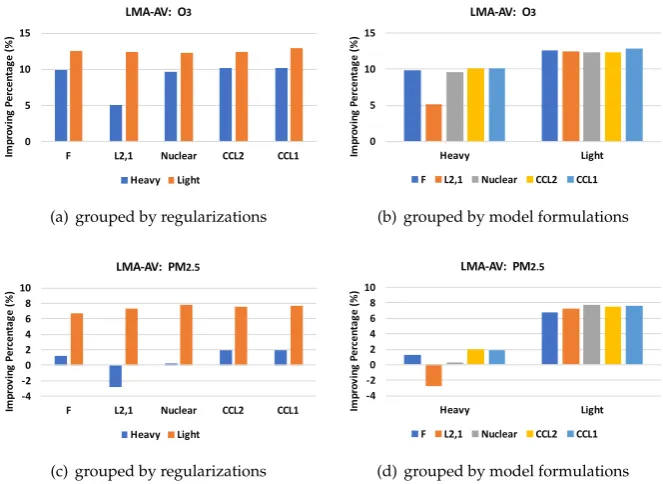
Figure 3.Improvement of Different Methods over the Baseline Method on LMA-AV dataset.
air pollutant of each dataset, we report two figures with one grouping the results by regularizations 268
and another one grouping the results by the model formulations. From the results, we can see 269
that (i) the light model formulation has clear advantage over the heavy model formulation and the 270
baseline model formulation, which implies that controlling the number of parameters is important for 271
improving generalization performance, and (ii) the proposed consecutive-close regularization yields 272
better performance than other regularizations, which verifies that considering the similarities between 273
models of consecutive hours are helpful. We also report the exact RMSE of each method in Table2. 274
Table 2.Root Mean Squared Error (RMSE) for all approaches and datasets
Approaches LMA-AV:O3 LMA-AV:PM2.5 LU-LV:O3 LU-LV:SO2
Baseline 0.1324 0.0399 0.0971 0.0334
Heavy-F 0.1193 0.0394 0.0882 0.0333
Heavy-L2, 1 0.12569 0.041 0.0883 0.033591
Heavy-Nuclear 0.1197 0.0398 0.0893 0.0333
Heavy CCL2 0.11896 0.0391 0.0882 0.033148
Heavy CCL1 0.11897 0.039134 0.0882 0.033261
Light-F 0.1158 0.0372 0.0848 0.0331
Light-L2,1 0.11591 0.037 0.085376 0.033411
Light-Nuclear 0.1161 0.0368 0.0849 0.0326
Light CCL2 0.116 0.0369 0.0845 0.03253
Light CCL1 0.11535 0.03684 0.085 0.03248
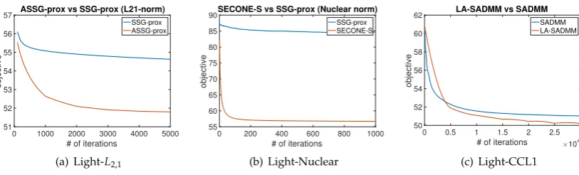
Finally, we compare the convergence speed of the employed optimization algorithms with their 275
standard counterparts. In particular, we compare ASSG vs SSG for optimizingL2,1regularized problem, 276
compare vs SSG for solving nulcear norm regularized problem, and compare with SADMM for solving 277
CC regularized problem. The results are plotted in Figure4, which demonstrates that the employed 278
0 1000 2000 3000 4000 5000 # of iterations
51 52 53 54 55 56 57
objective
ASSG-prox vs SSG-prox (L21-norm)
SSG-prox ASSG-prox
(a) Light-L2,1
0 200 400 600 800 1000
# of iterations 55
60 65 70 75 80 85 90
objective
SECONE-S vs SSG-prox (Nuclear norm) SSG-prox SECONE-S
(b) Light-Nuclear
0 0.5 1 1.5 2 2.5 3 # of iterations ×104 50
52 54 56 58 60 62
objective
LA-SADMM vs SADMM SADMM LA-SADMM
(c) Light-CCL1
Figure 4.Optimization techniques
6. Conclusions 280
In this paper, we have developed efficient machine learning methods for air pollutant prediction. 281
We formulated the problem as regularized multi-task learning and employed advanced optimization 282
algorithms for solving different formulations. We have focused on alleviating model complexity 283
by reducing the number of model parameters, and improving the performance by using structured 284
regularizer. Our results shows that the proposed light formulation achieves much better performance 285
than the other two model formulations, and the regularization by enforcing prediction models for two 286
consecutive hours to be close can also boost the performance of prediction. We have also shown that 287
advanced optimization techniques for important to improving the convergence of optimization and 288
speed up the training process for big data. For future work, we can further consider the commonalities 289
between nearby meteorology stations and combine them in a multi-task Learning framework, which 290
may further provide a boosting for the prediction. 291
References 292
1. Curtis, Luke, et al. "Adverse health effects of outdoor air pollutants."Environment international32.6 (2006):
293
815-830.
294
2. Mayer, Helmut. "Air pollution in cities."Atmospheric environment33.24 (1999): 4029-4037.
295
3. Samet, Jonathan M., et al. "The national morbidity, mortality, and air pollution study."Part II: morbidity and
296
mortality from air pollution in the United States Res Rep Health Eff Inst94.pt 2 (2000): 5-79.
297
4. Dockery, Douglas W., Joel Schwartz, and John D. Spengler. "Air pollution and daily mortality: associations
298
with particulates and acid aerosols."Environmental research59.2 (1992): 362-373.
299
5. Schwartz, Joel, and Douglas W. Dockery. "Increased mortality in Philadelphia associated with daily air
300
pollution concentrations."American review of respiratory disease145.3 (1992): 600-604.
301
6. American Lung Association.State of the air report. New York: ALA, (2007): 19-27.
302
7. Environmental Protection Agency, EPA (2009), Region 5: State Designations, as of September 18,
303
2009, available at https://archive.epa.gov/ozonedesignations/web/html/region5desig.html, accessed
304
12/17/2017.
305
8. Hinds, William C.Aerosol technology: properties, behavior, and measurement of airborne particles. John Wiley &
306
Sons,2012.
307
9. Soukup, Joleen M., and Susanne Becker. "Human alveolar macrophage responses to air pollution particulates
308
are associated with insoluble components of coarse material, including particulate endotoxin."Toxicology and
309
applied pharmacology171.1 (2001): 20-26.
310
10. Environmental Protection Agency, EPA CFR Parts 50, 51, 52, 53, and 58-National Ambient Air Quality
311
Standards for Particulate Matter: Final Rule. Fed. Regist, (2013), 78, 3086-3286.
312
11. Schwartz, Joel. "Short term fluctuations in air pollution and hospital admissions of the elderly for respiratory
313
disease."Thorax50.5 (1995): 531-538.
314
12. De Leon, A. Ponce, et al. "Effects of air pollution on daily hospital admissions for respiratory disease in
315
London between 1987-88 and 1991-92."Journal of Epidemiology & Community Health50.Suppl 1 (1996): s63-s70.
13. Birmili, Wolfram, and Alfred Wiedensohler. "New particle formation in the continental boundary layer:
317
Meteorological and gas phase parameter influence."Geophysical Research Letters27.20 (2000): 3325-3328.
318
14. Lee, Jong-Tae, et al. "Air pollution and asthma among children in Seoul, Korea."Epidemiology13.4 (2002):
319
481-484.
320
15. Cai, Changjie, et al. "Incorporation of new particle formation and early growth treatments into WRF/Chem:
321
Model improvement, evaluation, and impacts of anthropogenic aerosols over East Asia." Atmospheric
322
Environment124 (2016): 262-284.
323
16. Kalkstein, Laurence S., and Peter Corrigan. "A synoptic climatological approach for geographical analysis:
324
assessment of sulfur dioxide concentrations."Annals of the Association of American Geographers76.3 (1986):
325
381-395.
326
17. Comrie, Andrew C. "A synoptic climatology of rural ozone pollution at three forest sites in Pennsylvania."
327
Atmospheric Environment28.9 (1994): 1601-1614.
328
18. Eder, Brian K., Jerry M. Davis, and Peter Bloomfield. "An automated classification scheme designed to better
329
elucidate the dependence of ozone on meteorology."Journal of Applied Meteorology33.10 (1994): 1182-1199.
330
19. Zelenka, Michael P. "An analysis of the meteorological parameters affecting ambient concentrations of acid
331
aerosols in Uniontown, Pennsylvania."Atmospheric environment31.6 (1997): 869-878.
332
20. Laakso, Lauri, et al. "Diurnal and annual characteristics of particle mass and number concentrations in
333
urban, rural and Arctic environments in Finland."Atmospheric Environment37.19 (2003): 2629-2641.
334
21. Jacob, Daniel J., and Darrell A. Winner. "Effect of climate change on air quality."Atmospheric environment43.1
335
(2009): 51-63.
336
22. Holloway, Tracey, et al. "Change in ozone air pollution over Chicago associated with global climate change."
337
Journal of Geophysical Research: Atmospheres113.D22 (2008).
338
23. Akbari, Hashem. "Shade trees reduce building energy use and CO2 emissions from power plants." 339
Environmental pollution116 (2002): S119-S126.
340
24. DeGaetano, Arthur T., and Owen M. Doherty. "Temporal, spatial and meteorological variations in hourly
341
PM 2.5 concentration extremes in New York City."Atmospheric Environment38.11 (2004): 1547-1558.
342
25. Elminir, Hamdy K. "Dependence of urban air pollutants on meteorology."Science of the Total Environment
343
350.1 (2005): 225-237.
344
26. Natsagdorj, L., D. Jugder, and Y. S. Chung. "Analysis of dust storms observed in Mongolia during 1937?1999."
345
Atmospheric Environment37.9 (2003): 1401-1411.
346
27. Seinfeld, John H., and Spyros N. Pandis.Atmospheric chemistry and physics: from air pollution to climate change.
347
John Wiley & Sons,2016.
348
28. Koschmieder, Harald. "Theorie der horizontalen Sichtweite."Beitrage zur Physik der freien Atmosphare(1924):
349
33-53.
350
29. Appel, B. R., et al. "Visibility as related to atmospheric aerosol constituents."Atmospheric Environment(1967)
351
19.9 (1985): 1525-1534.
352
30. Deng, Xuejiao, et al. "Long-term trend of visibility and its characterizations in the Pearl River Delta (PRD)
353
region, China."Atmospheric Environment42.7 (2008): 1424-1435.
354
31. Twomey, Sean. "The influence of pollution on the shortwave albedo of clouds."Journal of the atmospheric
355
sciences34.7 (1977): 1149-1152.
356
32. Zhuoning Yuan, Xun Zhou, Tianbao Yang, James Tamerius, Ricardo Mantilla. Predicting Traffic Accidents
357
Through Heterogeneous Urban Data: A Case Study. In 6th International Workshop on Urban Computing
358
(UrbComp 2017) in conjunction with ACM KDD2017 359
33. Zheng, Yu, Furui Liu, and Hsun-Ping Hsieh. "U-Air: When urban air quality inference meets big data."
360
Proceedings of the 19th ACM SIGKDD international conference on Knowledge discovery and data mining. ACM,
361
2013.
362
34. Kalapanidas, Elias, and Nikolaos Avouris. "Short-term air quality prediction using a case-based classifier."
363
Environmental Modelling & Software16.3 (2001): 263-272.
364
35. Athanasiadis, Ioannis N., et al. "Applying machine learning techniques on air quality data for real-time
365
decision support."First international NAISO symposium on information technologies in environmental engineering
366
(ITEE’2003), Gdansk, Poland.2003.
367
36. Singh, Kunwar P., Shikha Gupta, and Premanjali Rai. "Identifying pollution sources and predicting urban air
368
quality using ensemble learning methods."Atmospheric Environment80 (2013): 426-437.
37. Corani, Giorgio. "Air quality prediction in Milan: feed-forward neural networks, pruned neural networks
370
and lazy learning."Ecological Modelling185.2 (2005): 513-529.
371
38. Fu, Minglei, et al. "Prediction of particular matter concentrations by developed feed-forward neural network
372
with rolling mechanism and gray model."Neural Computing and Applications26.8 (2015): 1789-1797.
373
39. Jiang, Dahe, et al. "Progress in developing an ANN model for air pollution index forecast."Atmospheric
374
Environment38.40 (2004): 7055-7064.
375
40. Ni, X. Y., H. Huang, and W. P. Du. "Relevance analysis and short-term prediction of PM 2.5 concentrations in
376
Beijing based on multi-source data."Atmospheric Environment150 (2017): 146-161.
377
41. Caruana, Rich. "Multitask learning."Learning to learn. Springer US,1998. 95-133.
378
42. Collobert, Ronan, and Jason Weston. "A unified architecture for natural language processing: Deep neural
379
networks with multitask learning."Proceedings of the 25th international conference on Machine learning. ACM,
380
2008.
381
43. Fan, Jianping, Yuli Gao, and Hangzai Luo. "Integrating concept ontology and multitask learning to achieve
382
more effective classifier training for multilevel image annotation."IEEE Transactions on Image Processing17.3
383
(2008): 407-426.
384
44. Widmer, Christian, et al. "Leveraging Sequence Classification by Taxonomy-Based Multitask Learning."
385
RECOMB.2010.
386
45. Kshirsagar, Meghana, Jaime Carbonell, and Judith Klein-Seetharaman. "Multitask learning for host-pathogen
387
protein interactions."Bioinformatics29.13 (2013): i217-i226.
388
46. Lindbeck, Assar, and Dennis J. Snower. "Multitask learning and the reorganization of work: From tayloristic
389
to holistic organization."Journal of labor economics18.3 (2000): 353-376.
390
47. Liu, Jun, Shuiwang Ji, and Jieping Ye. "Multi-task feature learning via efficient l 2, 1-norm minimization."
391
Proceedings of the twenty-fifth conference on uncertainty in artificial intelligence. AUAI Press,2009.
392
48. Recht, Benjamin, Maryam Fazel, and Pablo A. Parrilo. "Guaranteed minimum-rank solutions of linear matrix
393
equations via nuclear norm minimization."SIAM review52.3 (2010): 471-501.
394
49. Argyriou, Andreas, Charles A. Micchelli, and Massimiliano Pontil. "On spectral learning."Journal of Machine
395
Learning Research11.Feb (2010): 935-953.
396
50. Maurer, Andreas. "Bounds for linear multi-task learning."Journal of Machine Learning Research7.Jan (2006):
397
117-139.
398
51. Foley, K. M., et al. "Incremental testing of the Community Multiscale Air Quality (CMAQ) modeling system
399
version 4.7."Geoscientific Model Development3.1 (2010): 205.
400
52. Yahya, Khairunnisa, et al. "Decadal application of WRF/Chem for regional air quality and climate modeling
401
over the US under the representative concentration pathways scenarios. Part 1: Model evaluation and
402
impact of downscaling."Atmospheric Environment152 (2017): 562-583.
403
53. Horel, John, et al. "Mesowest: Cooperative mesonets in the western United States."Bulletin of the American
404
Meteorological Society83.2 (2002): 211-225.
405
54. Zhang, Tong. "Solving large scale linear prediction problems using stochastic gradient descent algorithms."
406
Proceedings of the twenty-first international conference on Machine learning. ACM,2004.
407
55. Xu, Yi, Qihang Lin, and Tianbao Yang. "Stochastic Convex Optimization: Faster Local Growth Implies Faster
408
Global Convergence."International Conference on Machine Learning.2017.
409
56. Parikh, Neal, and Stephen Boyd. "Proximal algorithms."Foundations and Trends in Optimization1.3 (2014):
410
127-239.
411
57. Xiao, Yichi, et al. "SVD-free Convex-Concave Approaches for Nuclear Norm Regularization."IJCAI.2017.
412
58. Xu, Yi, et al. "ADMM without a Fixed Penalty Parameter: Faster Convergence with New Adaptive
413
Penalization."Advances in Neural Information Processing Systems.2017.