Multiscale Modelling Of Platelet Aggregation

University of Pennsylvania

ScholarlyCommons

Publicly Accessible Penn Dissertations

2017

Multiscale Modelling Of Platelet Aggregation

Yichen Lu

University of Pennsylvania, [email protected]

Follow this and additional works at:https://repository.upenn.edu/edissertations

Part of theChemical Engineering Commons

This paper is posted at ScholarlyCommons.https://repository.upenn.edu/edissertations/2452

For more information, please [email protected].

Recommended Citation

Lu, Yichen, "Multiscale Modelling Of Platelet Aggregation" (2017).Publicly Accessible Penn Dissertations. 2452.

Multiscale Modelling Of Platelet Aggregation

Abstract

During clotting under flow, platelets bind and activate on collagen and release autocrinic factors such ADP and thromboxane, while tissue factor (TF) on the damaged wall leads to localized thrombin generation. Toward patient-specific simulation of thrombosis, a multiscale approach was developed to account for: platelet signaling (neural network trained by pairwise agonist scanning, PAS-NN), platelet positions (lattice kinetic Monte Carlo, LKMC), wall-generated thrombin and platelet-released ADP/thromboxane convection-diffusion (PDE), and flow over a growing clot (lattice Boltzmann). LKMC included shear-driven platelet aggregate restructuring. The PDEs for thrombin, ADP, and thromboxane were solved by finite element method using cell activation-driven adaptive triangular meshing. At all times, intracellular calcium was known for each platelet by PAS-NN in response to its unique exposure to local collagen, ADP, thromboxane, and thrombin. The model accurately predicted clot morphology and growth with time on collagen/TF surface as compared to microfluidic blood perfusion experiments. The model also predicted the complete occlusion of the blood channel under pressure relief settings.

Prior to occlusion, intrathrombus concentrations reached 50 nM thrombin, ~1 μM thromboxane, and ~10 μM ADP, while the wall shear rate on the rough clot peaked at ~1000-2000 sec-1. Additionally, clotting on TF/collagen was accurately simulated for modulators of platelet cyclooxygenase-1, P2Y1, and IP-receptor. The model was then extended to a rectangular channel with symmetric Gaussian obstacles representative of a coronary artery with severe stenosis. The upgraded stenosis model was able to predict platelet deposition dynamics at the post-stenotic segment corresponding to development of artery thrombosis prior to severe myocardial infarction. The presence of stenosis conditions alters the hemodynamics of normal hemostasis, showing a different thrombus growth mechanism. The model was able to recreate the platelet aggregation process under the complex recirculating flow features and make reasonable prediction on the clot morphology with flow separation. The model also detected recirculating transport dynamics for diffusible species in response to vortex features, posing interesting questions on the interplay between biological signaling and prevailing hemodynamics. In future work, the model will be extended to clot growth with a patient cardio-vasculature under pulsatile flow conditions.

Degree Type

Dissertation

Degree Name

Doctor of Philosophy (PhD)

Graduate Group

Chemical and Biomolecular Engineering

First Advisor

Scott L. Diamond

Second Advisor

Talid R. Sinno

Keywords

Multiscale Modelling, Neural Network, Platelet Aggregation, Stenosis, Thrombosis

Subject Categories

Chemical Engineering

MULTISCALE MODELLING OF PLATELET AGGREGATION

Yichen Lu

A DISSERTATION in

Chemical and Biomolecular Engineering

Presented to the Faculties of the University of Pennsylvania In Partial Fulfillment of the Requirements for the

Degree of Doctor of Philosophy 2017

Co-Supervisor of Dissertation Co-Supervisor of Dissertation

_________________________ _________________________ Scott L. Diamond, Professor Talid R. Sinno, Professor

Chemical and Biomolecular Engineering Chemical and Biomolecular Engineering

Graduate Group Chairperson

_________________________ John C. Crocker, Professor Chemical and Biomolecular Engineering

Dissertation Committee

MULTISCALE MODELLING OF PLATELET AGGREGATION

COPYRIGHT

2017

iii

ACKNOWLEDGMENT

First and foremost, I would like to express my sincere gratitude to two advisors of mine Professor Scott Diamond and Professor Talid Sinno for their continuous guidance through my entire PhD study. I feel privileged to be a student of these great advisors who have demonstrated patience, enthusiasm and wisdom. I cherish every moment of our precious discussion about the direction of research. To me, it is an incredible learning experience to tackle challenging questions together with two wise scholars from different backgrounds.

I would also like to thank for Dr. John Crocker and Dr. Lawrence Brass for serving as committee members. Their constructive criticism greatly broadened the horizon of the project. I really appreciate their insightful comments and continuous encouragement. In my daily work I have been blessed with a friendly and cheerful group of fellow students. I would like to extend my gratitude to the company of all the fellow labmates have stayed on the fifth floor of Vagelos: Andrew, Mei, Yungchi, Ian, Danny, Jifu, Anand, Mehdi, Evan for the meaningful conservations and discussions. The same goes to all other lab members of both Sinno and Diamond for their insightful comments on research and life in general.

iv

v

ABSTRACT

MULTISCALE MODELLING OF PLATELET AGGREGATION

Yichen Lu

Scott L. Diamond

Talid R. Sinno

vi

modulators of platelet cyclooxygenase-1, P2Y1, and IP-receptor. The model was then

vii

TABLE OF CONTENT

ACKNOWLEDGMENT ... III

ABSTRACT ... V

TABLE OF CONTENT ... VII

LIST OF TABLES ... X

LIST OF ILLUSTRATIONS ... XI

CHAPTER 1 : INTRODUCTION ... 1

1.1 Background of hemostasis and thrombosis ... 4

1.2 Blood coagulation cascade ... 6

1.3 Microfluidic models of thrombosis in flow ... 7

1.4 Numerical models of platelet aggregation and blood coagulation ... 8

CHAPTER 2 : NUMERICAL METHODS ... 14

2.1 Kinetic Monte Carlo method for stochastic systems ... 15

2.1.1 System update method ... 16

2.1.2 Lattice Kinetic Monte Carlo for diffusion and convection ... 17

2.2 Lattice Boltzmann method for perturbed flow ... 21

2.2.1 Streaming and collision propagator ... 22

2.2.2 Boundary conditions ... 24

2.3 Finite element method for diffusive agonist transport ... 25

2.4 Neural network ... 27

CHAPTER 3 MULTISCALE MODELLING OF PLATELET AGGREGATION . 30 3.1 Introduction ... 30

3.2 Experimental methods ... 35

3.2.1 Introduction of platelet activation and calcium measurement ... 35

3.2.2 Pairwise agonist scanning and neural network training ... 37

viii

3.2.3 Blood collection and preparation ... 40

3.2.4 Preparation and characterization of collagen/TF surface ... 41

3.2.5 Microfluidic clotting assay on collagen surfaces with or without TF ... 42

3.2.6 Confocal imaging of clot morphology and flow rate ... 43

3.2 Model specification ... 44

3.2.1 Schematics of the multiscale model ... 44

3.2.2 Kinetic Monte Carlo... 48

3.2.3 Lattice Boltzmann ... 52

3.2.3 Finite Element method ... 54

3.2.4 Cell activation-driven adaptive meshing ... 55

3.2.5 Neural Network ... 65

3.2.6 Thrombin release modeled as boundary flux ... 67

3.2.7 Clot remodeling scheme ... 71

3.2.8 Module integration ... 73

3.3 Results ... 77

3.3.1 Cell activation-driven adaptive meshing ... 77

3.3.2 Thrombin flux case studies ... 79

3.3.3 Platelet remodeling upon deposition and thrombus morphology ... 84

3.3.4 Constant Flow and Pressure Relief ... 87

3.3.5 Agonist study ... 91

3.4 Discussion ... 92

3.5 Conclusion ... 96

CHAPTER 4 : PLATELET AGGREGATION UNDER STENOTIC CONDITIONS ... 99

4.1 Introduction ... 99

4.2 Stabilization techniques for Finite Element method ... 101

4.2.1 The Streamline Upwind Petrov-Galerkin (SUPG) method ... 101

4.2.2 Spurious Oscillations at Layers Diminishing (SOLD) methods ... 104

4.2.3 FEM-flux corrected transport (FEM-FCT) schemes ... 106

4.3 Simulation methods ... 109

4.3.1 Creation of stenosis geometry ... 110

4.3.2 Lattice Kinetic Monte Carlo for stenosis simulation ... 111

4.3.3 Lattice Boltzmann for complex flow recirculation ... 112

4.3.4 Stabilized finite element calculation ... 113

4.4 Results ... 114

4.4.1 Flow within a stenotic channel ... 114

4.4.2 Platelet trajectory under stenosis ... 117

4.4.3 Thrombus development under stenosis ... 118

4.4.4 Transport of diffusible agonists under stenosis ... 121

ix

CHAPTER 5 : FUTURE WORK ... 127

5.1 Model for fibrin polymerization ... 127

5.2 Model for bleeding... 130

5.3 Model for patients with coronary artery diseases... 130

5.4 Model optimization... 132

CHAPTER 6 : TIME COURSE OF SIMULATION ... 133

x

LIST OF TABLES

xi

LIST OF ILLUSTRATIONS

Figure 1-1: Schematic of simplified model of the coagulation cascade ... 7

Figure 2-1: Illustration of the KMC algorithm ... 18

Figure 2-2: Illustration of the Pass Forward Algorithm... 19

Figure 2-3: Example of discretized spherical platelets ... 20

Figure 2-4: D2Q9 unit node including 8 nearest neighbors and itself ... 22

Figure 2-5: A simple neural network structure with p inputs and single output... 28

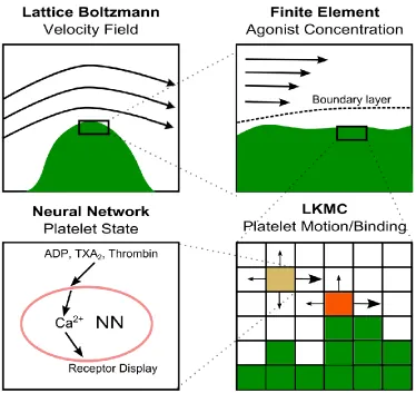
Figure 3-1: Multiscale picture of computational modules (Lattice Boltzmann for flow field, Finite Element for agonist concentration, Neural Network for calcium prediction, Lattice Kinetic Monte Carlo for platelet motion) ... 32

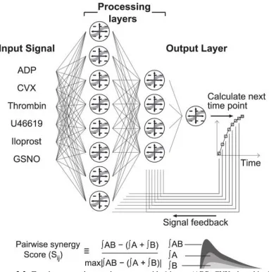
Figure 3-2: Two-layer neural network structure with 6 inputs (ADP, CVX, thrombin, U46619, Iloprost, GSNO) to predict platelet calcium trace... 33

Figure 3-3: Platelet calcium pathway involving six agonists (ADP, U46619, convulxin, thrombin, iloprost, GSNO) ... 37

Figure 3-4 Neural network fit of PAS experiments. ... 40

Figure 3-5: The 8-channel microfluidic device and epifluorescence microscopy (A,B). . 42

Figure 3-6: The simulation domain in comparison with the microfluidic device... 44

Figure 3-7: Multiscale model coupling ... 46

Figure 3-8: Simulation domains and meshes for the different modules. ... 47

Figure 3-9: Inlet platelet concentration distribution and drift velocity. ... 49

Figure 3-10: Initial shear distribution for the pressure relief experimental settings. ... 53

Figure 3-11: Platelet activation-driven adaptive triangular meshing ... 56

Figure 3-12: Flowchart for the DistMesh algorithm ... 59

Figure 3-13: Mesh configuration at 20 seconds ... 61

Figure 3-14: Mesh configuration at 100 seconds ... 62

Figure 3-15: Mesh configuration at 200 seconds ... 63

Figure 3-16: Mesh configuration at 300 seconds ... 64

Figure 3-17 Comparison of different thrombin flux signals for constant flow rate simulations at initial inlet wall shear rate = 200 s-1. ... 70

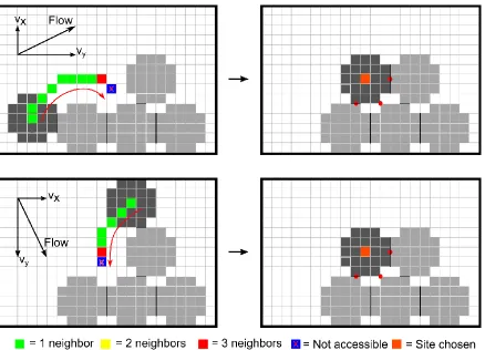
Figure 3-18: Remodeling algorithm for platelet deposition. ... 72

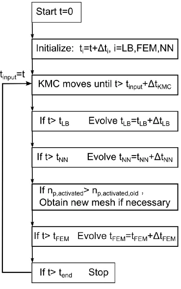
Figure 3-19: Multiscale model time stepping ... 74

Figure 3-20: Histogram for mesh quality obtained by the adaptive meshing scheme. Most of the triangular elements had very high mesh quality (>0.9). ... 78

Figure 3-21: Calcium signaling predicted by neural network for platelets exposed to different agonists within the thrombus. ... 81

Figure 3-22: Comparison of experiment (A,C) and multiscale simulation (B,D). ... 82

Figure 3-23: Fully resolved thrombosis for whole blood flow over collagen/TF after 400 sec. ... 83

Figure 3-24: Comparison of thrombus morphology with and without the remodeling algorithm. The remodeling algorithm resulted in physically realistic clot morphology (bottom) as compared to the highly dendritic and mechanically unlikely structure obtained without remodeling upon adhesion (top). ... 85

xii

Figure 3-26 Evolution over 400 sec of flow and thrombosis (ADP, TXA2, thrombin) at

constant flow rate (A) or pressure relief mode (B). Initial inlet wall shear rate = 200 s-1.

... 90

Figure 3-27: Comparison of experiment (A) and multiscale simulation (B) for different agonist conditions. ... 92

Figure 3-28: Connection between experimental measurement and numerical prediction 98 Figure 4-1 Comparison of the microfluidic channel and coronary artery ... 109

Figure 4-2: Flow field with vortex feature obtained with maximum axial velocity at the inlet = 2.2cm/s ... 116

Figure 4-3: Axial velocity distribution at the different locations ... 116

Figure 4-4: Trajectory of platelets at different axial locations ... 118

Figure 4-5: Development of thrombus at the post-stenotic arch ... 120

Figure 4-6: Concentration field for ADP, TXA2, IIa for stenotic channel ... 122

Figure 5-1 Thrombin flux from clots growing on collagen/TF ... 129

Figure 6-1: Multiscale simulation of platelet deposition under constant flow mode at 1 sec ... 133

Figure 6-2: Multiscale simulation of platelet deposition under constant flow mode at 100 sec. ... 134

Figure 6-3: Multiscale simulation of platelet deposition under constant flow mode at 200 sec. ... 135

Figure 6-4: Multiscale simulation of platelet deposition under constant flow mode at 300 sec. ... 136

Figure 6-5: Multiscale simulation of platelet deposition under constant flow mode at 400 sec. ... 137

Figure 6-6: Multiscale simulation of platelet deposition under pressure relief mode at 1 sec. ... 138

Figure 6-7: Multiscale simulation of platelet deposition under pressure relief mode at 100 sec. ... 139

Figure 6-8: Multiscale simulation of platelet deposition under pressure relief mode at 200 sec. ... 140

Figure 6-9: Multiscale simulation of platelet deposition under pressure relief mode at 300 sec. ... 141

1

Chapter 1: Introduction

2

the drug dosage based on the genetic fingerprints of certain stratification of patient groups.

3

different levels. This gives rise to a lot of interesting challenges in model integration and algorithm optimization. More importantly, numerical models can never be built without essential knowledge derived from experiments. Experimental data typical serve as guidance in identifying crucial mechanisms and important subcomponents. The experimental measure will be essential for calibration and validation of models. Models on the other hand can be extremely usefully in generating hypothesis and predicting behaviors outside the experimental dataset, which adds to the understanding of the biological principles even further.

4

of biological mechanisms and physical forces that naturally call for a multiscale modelling approach.

The rest of the thesis will be focused on building a multiscale platelet aggregation model to simulate the process of clot formation under blood flow. The following sections in Chapter 1 will provide a general overview of the background for platelet aggregation and blood coagulation with an emphasis on model development. Chapter 2 will discuss a number of numerical techniques for building the multiscale model. Chapter 3 will focus on the detailed description of the multi-component lattice Kinetic Monte Carlo (LKMC) model to simulate the stochastic motion and reaction of platelets within a microfluidic channel. In Chapter 4, the model will be extended to a representative coronary artery with stenotic geometry. Finally, Chapter 5 will discuss the potential future application and improvement of the model.

1.1 Background of hemostasis and thrombosis

5

fully spread cells and start to release autocrine activators such as ADP and thromboxane (TXA2). [4] These diffusive secondary pro-coagulant agonists play a significant role in

biological signaling by recruiting quiescent and activating new platelets to the injury site. Apart from collagen and vWF, the exposed tissue factor initiates the coagulation cascade, producing an important serine protease known as thrombin. Thrombin executes several critical reactions involving cleavage of fibrinogen to insoluble fibrin [5], cleavage of PAR1 and PAR4 to initiate platelet activation [6], feedback activation of zymogens such as factor XI, VIII and V. [5]

Thrombosis refers to pathological clot formation, causing complete occlusion of blood vessels leading to life-threatening events of myocardial infarction, stroke and venous thromboembolism. In fact, acute atrial thrombosis is the responsible for more than 90% of myocardial infarction and stokes, which are the two major causes of death in the western world. [7] The treatment of arterial thrombosis is generally realized by inhibition of platelet aggregation through many drug targets. [8] Clopidogrel blocks the receptor P2Y12, thereby inhibiting the activation of adenosine diphosphate. [9] Acetylsalicylic acid (aspirin) irreversibly inhibits COX-1 in the thromboxane A2 synthesis pathway, therefore inhibiting the activation of TXA2. [10] There are also intravenous (IV) drugs

6

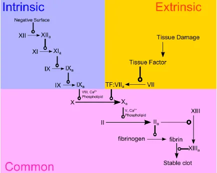
1.2 Blood coagulation cascade

7

Figure 1-1: Schematic of simplified cascades in the blood coagulation cascade

1.3 Microfluidic models of thrombosis in flow

8

Recently, microfluidic devices have been fabricated [16-19] to generate an open reacting reservoir with blood being directed into the microfluidic channels. Strips of collagen are laid perpendicular to the microfluidic channels to mimic a focal injury. The 8-channel microfluidic devices allow for generation of large datasets where different conditions can be tested in different channels for one single experiment. Direct imaging of platelet deposition can be done in the microfluidic channels with fluorescence microscopy, and morphological information can also be extracted. [20] For studies of thrombin generation, tissue factors can also be affixed to the surface of the microfluidic channel. Colace et al. [21] linked TF-incorporated lipid liposomes to collagen surface by iotinavidin interaction to create prothrombotic surfaces mimicking in vivo injuries. Local hemodynamic conditions can be perfectly replicated among 8 channels to quantify thrombus formation dynamics with and without fibrin deposition. The high-throughput nature of the device has also enabled the manipulation of various drug conditions and has been applied to study patients with congenital bleeding disorders. [22]

1.4 Numerical models of platelet aggregation and blood coagulation

Models for platelet signaling

9

both steady-state and dynamical information in determining the platelet activation function. A more recent effort is to use artificial neural network to characterize the signaling pathways. Rather than directly estimating the kinetic parameters and reaction mechanisms, the neural network (NN) predicts the intracellular calcium response by creating artificial network architecture. The NN is mainly data-driven and focuses on the final output without resolving the intermediate processes. Chatterjee et al. used high-throughput, pairwise agonist scanning method to obtain calcium response to binary simulation of agonists at different concentration levels. The NN was then be trained with carefully designed parameterized architecture and validated with similar datasets. The NN allows for patient-specific prediction on the platelet signaling.[25] Later, Lee el al. further expanded the NN model to 6 agonists, including thrombin. The work characterized an averaged calcium response function based on training data collected from 10 healthy donors. One thing to note is that all these models assumed the homogeneous well-mixed condition where only prediction on the averaged calcium response. [26]

Models for coagulation cascade

10

to include the activation state of platelets. The activated platelet state is used as a modulator for reaction rates within the coagulation cascade. The development of concentration of the coagulation factors was predicted and validated against combinatorial high-throughput experiment. [29] The goal of these ODE models aims to obtain thrombin generation function in response to different levels of tissue factor simulation. Again, the assumption of the ODE formulation is reliant on all species being homogenous within the system. The predicted thrombin generation curve typically has an initiation phase followed by a decaying stage as thrombin inhibition takes place.

Models for particle motion under flow

11

particles. Such models include dissipative particle dynamic (DPD) model [30], the cellular Potts model [37], the lattice Kinetic Monte Carlo model with convection[38,39]. Flamm extended the limit of traditional kinetic Monte Carlo method to include the effect of convective field. Later the model was further extended to include aggregation reaction. These methods can cover a much longer time scale, thus are well-suited for simulations of platelet motion under flow.

Models for particle margination

Platelet margination refers to the process of small platelets being pushed to the vessels of other large particles such as red blood cells under hydrodynamics forces. Platelets experience a shear-induced diffusion (SID) which describes the motion of particles in a flowing suspension due to collision with large particles [40]. The collisions are caused by gradients in particle density and suspending fluid viscosity that lead to the motion of particles in the flow direction and perpendicular to it. It was found the effective diffusivity from solute transport model with red blood cells was O(10-7) cm2/s [41], while the diffusion coefficient estimated from the Stokes-Einstein equation was O(10-9) cm2/s. This indicates the classical Brownian motion can be neglected and the platelets motion results mostly from their interaction with RBCs or the perturbation of suspending fluid by large cellular entities.[42]

12

proposed by Eckstein and Belgacem [40]. Later Yeh proposed a spatially varying drift velocity determined by experimental data [43]. Chen et al. proposed a formulation for the radial drift by considering the effective radii of both RBC and platelet and also the RBC collision gradient [44].

Fully coupled multiscale models for platelet aggregation

To under the entire clotting process, a multiscale modelling approach has to be adopted to account for aspects like platelet adhesion and aggregation, blood coagulation initiated by tissue factor, release of secondary agonists, and platelet signaling. A fully coupled model will require interaction between different numerical techniques across many disciplines with involve spatial scales ranging from millimeters to nanometers and timescales from minutes to milliseconds.

The past decade has witnessed an upsurge of new models describing the clotting process with fully resolved particle-fluid interaction. In the meantime, there is an occurrence of a wealth experimental data both from in vitro microfluidic perfusion [16,18,20] and in vitro injury models [45-47].

Leiderman and Fogelson used a continuum method based on immerse boundary method [48] that explicitly solves the spatial-temporal variations of agonists. The Leiderman-Fogelson model treated platelets (inactivated and activated) of continuum species and made prediction on thrombin generation by solving kinetics and transport of zymogens and enzymes.

13

nodes, where the transformation between two nodes is achieved by specifying a Hamiltonian where a Metropolis Monte Carlo criterion was used to accept or reject any move.

Flamm et al. [49] developed a lattice Kinetic Monte Carlo model that used kinetic Monte Carlo to solve platelet motion, lattice Boltzmann for fluid flow, finite element to solve transport of diffusive agonists. The platelet signaling was characterized an artificial neural network trained from patient data. The Flamm model didn’t consider the thrombin generation.

14

Chapter 2: Numerical Methods

15

2.1 Kinetic Monte Carlo method for stochastic systems

Kinetic Monte Carlo (kMC) algorithm is an extension to the classic Metropolis Monte Carlo methods where the evolution of systems is governed by a series of randomly sampled events that satisfy the desired overall kinetics. KMC aims to evolve the system dynamically from state to state by pre-calculating all possible transition rates for the current configuration with time increments congruent with the underlying microscopic kinetics of the system. Unlike Molecular Dynamics (MD) which can typically reproduce the dynamics of the system of time scale less than 10 nanoseconds, kMC simulations can usually reach seconds and well beyond. [51]

A typical simulation has three major steps:

1. Choose next event based on pre-calculated rate information 2. Update the system clock according to the specific event 3. Update rate catalog following event execution

The wait time after one event is being executed can be calculated from the assumption that all events are independent Poisson processes. More specifically, let





P   be the joint distribution of the next event being time μ and occurring in the time

interval









 









 

0 total

P    t , where

1

N total i

i

 



executed is of type  and occurs in the time interval









16

The wait time for the next event for N independent Poisson processes is ln

 

total u

  

 ,

where u is a random number drawn from the unit interval, with _average 1

total

 

 . And the

probability of choosing event μ as the next event is

total P_  

 .

2.1.1 System update method

There are three typical system update method based on the kMC probability schemes. Gillespie first proposed direct method where for each step, a specific event was determined by the random number u and by locating the exact event number μ satisfying

1

1 1

i i

i total i total

u          





update. Gillespie then proposed an improved first reaction method by directly sampling random wait times for all events. More specifically, for each event i, a wait time is

randomly generated with _i ln

 

i u

  

 . As Poisson processes are memoryless, it is only

17

events which can be obtained with O(log(N)) with efficient sorting algorithms such as skip list, quick sort, etc.

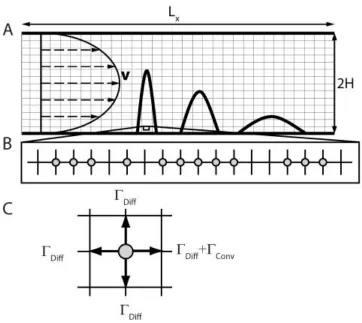
2.1.2 Lattice Kinetic Monte Carlo for diffusion and convection

Flamm, et al proposed a lattice kinetic Monte Carlo algorithm that simulates the trajectories of tracer particle in the fluid undergoing diffusive and convective motion. [39] To implement LKMC, the important input is the rate catalog summarizing probabilities of all possible events. The simulation domain is typically discretized with uniform lattice spacing in each direction of motion (Figure 2-1A, B). The reaction rate for a diffusive

move from one lattice site to its nearest neighbor is defined as d ₂ D h

  , where h is the

lattice spacing and D is isotropic diffusivity . The rate of a convective motion in the

direction i is given by i c

v h

  . The combined diffusive and convective motion rates in

the direction i is i ₂ motion

v D

h h

   (Figure 2-1C). In the case of blockage, this Simplest

18

Figure 2-1: Illustration of the KMC algorithm

(a) Two-dimensional rectangular domain discretized with lattice spacing hx and hy. The flow field,

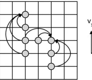
19

Figure 2-2: Illustration of the Pass Forward Algorithm

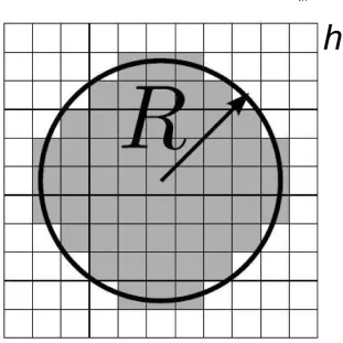
20

The lattice spacing is typically not restricted the size of particle. A particle can take up

several lattices and we can define the radial resolution R h

  as the ratio of the particle

radius R and lattice spacing h. (Figure 2-3) It has been shown that in the low

concentration limit, the algorithmic diffusive error due to discretization is

2

err vh D  The

numerical error Peclet number is defined as _LKMC 2

err vR Pe

D 

  .

Figure 2-3: Example of discretized spherical platelets

A platelet of radius R is placed on a uniform grip of size h with radial resolution R

h

21

2.2 Lattice Boltzmann method for perturbed flow

22

2.2.1 Streaming and collision propagator

Almost all incompressible fluid problems can be reduced to solving the Navier-Stokes equation with continuity constraints where the velocity field vsatisfies:

2 2

0

P

t 



      

 

v

v v v

v

, (2-1)

where is the kinematic viscosity of the fluid.

The simulation domain is discretized to uniform square lattices where a unit cell contains several lattice directions.

Figure 2-4: D2Q9 unit node including 8 nearest neighbors and itself

23 0

0

1 0 1 0

0 1 0 1

1 1 1 1

1 1 1 1

                _{ } _{ } _{ } _{ }                    _{ } _{ } _{ } _{ }           0

1 2 3 4

5 6 7 8

e

e e e e

e e e e

(2-2)

and _x_y 1 for lattice space, _t 1 for time step. The probability distribution of particle at a node position x at time t with velocity e_iis denoted as f_i

 





 



 



i i i

f x e _i t  t f x t   f x t i (2-3)

The density and momentum are defined as moments of the distribution function satisfying:

,

i i

i i

f f

 





and conservation of mass and momentum:

0, 0

i i

i i

   





One popular propagator known as the Bhatnaar, Gross and Krook (BGK) operator [53] involving single relaxation parameter  is defined as:

 

 





1

, eq ,

i _ fi t fi t

   x  x , (2-6)

24

equivalent solution time is reached. The exact formulation for D2Q9 is summarized as follows:

The equilibrium distribution is









2 2

eq i i

f w_      _

 e vi e vi v  (2-7)

where the weights are

0 1 2 3 4 5 6 7 8

4 1 1

, ,

9 9 36

w  w w w w  w w w w  (2-8)

Propagation step:





 

*

, ,

i i

f x e _i t  f x t (2-9)

The BGK formula for collision:





 



 

 



, , , eq ,

i i i i

f t t f t f t f t



 _i      

x e x x x (2-10)

where *

 

,

eq i

f x t is the post-propagation/pre-collision equilibrium distribution and the

relaxation parameter  (typically between 0.5 to 2.0) is related to kinetic viscosity in LB

unit 6 1

2

LB



   .

2.2.2 Boundary conditions

25

setting a constraint on the density function rather than the velocity component usually at the both the inlet and outlet. For a fully discretized system where the boundary nodes coincide with the obstacle, usually some variants of the classic bounce-back rules are applied. For more complicated cases where hierarchical gridding schemes are applied, the unaligned nodal structures call for special treatment where half bounce-back rules or curve boundary-conditions [54] are utilized. In the case of advanced flow propagator which allows multiple relaxation parameters, boundary conditions need to be changed accordingly to avoid unphysical representation in distribution function with more than relaxation times.

2.3 Finite element method for diffusive agonist transport

Finite element method (FEM) is a simple yet powerful method to solve numerical partial differential equations relating to the transport of reactive-diffusive agonists under complex flow conditions. The governing equation solving the concentration field C for a soluble species known as the convective-diffusion-reaction equations is given by

2

C

C D C R

t

 _{    }

 v (2-11)

where v is velocity field of the fluid, D is the diffusion coefficient of the solute, and R is the generation/consumption rate for the solvent.

26 field C pertaining to element e is

1 ˆ e e

i i i

C  C







i is adjacent to the element e. The original PDE can be reduced to simple linear matrix system due to the linearity in the FEM method. The weight residual for the ith node, Wi

has to be balanced for any piecewise interpolation of the basis function _i. Therefore

2

i i i i

C

W d W Cd W D Cd W Rd

t

   

 _{        }











which by Green’s theorem reduces to

i i

i i i i

C

d Cd

t

D Cd D C d Rd

                            











C C

 



i i j j

j j

n n

i i j j i j j i

j j

C

d C d

t

D C d D C d Rd

                                  



















The reduced matrix system is given by,



M C+ AC = b (2-15)

27





 

 

e e e ij i j i j

e

e e e

ij i j i j

e

e e e

ij i j i j

e

e e e

i i i j

e e

i i i

e

C C C

C

C C

t t t

M d d

K D d D d

G d d

p C d C d

r Rd Rd

                                  _{   } _                               































Generally a finite difference approximation is applied to the time

derivative 1 t t t t   _   

C C C

. A weighted contribution from the previous time and the

current time is applied to the matrix A and the vector b.









1  t  t , 1  t  t

     

A A A b b b (2-17)

If 0, the explicit Euler method is obtained.  1 gives the implicit Euler method,

which is unconditionally stable. If 1

2

  , the Crank-Nicolson method is obtained.

2.4 Neural network

28

activation information to the next layer and making prediction based on the overall additive response from other nodes.

Figure 2-5: A simple neural network structure with p inputs and single output

A naive neural network structure is shown in (Figure 2-5), which is equivalent to a multiple linear regression model in which the expected response y is related to the values of inputs x





0 1

p i i i

y w w x



 



The one single processing node in this case, translates the information by simply using a linear combination of all different input variables with a bias term with weights left to be determined through an optimization process. The major step of constructing a neural network involves:

1. Design the architecture of the artificial network. 2. Propose appropriate activation and loss function.

3. Obtain unknown weights through iterative gradient search over the parameter spaces.

y

0

w



1

x

2

x

p

29

30

Chapter 3Multiscale modelling of platelet aggregation

3.1 Introduction

Platelets play a critical role in primary hemostasis to prevent blood loss due to vessel injury. Secondary hemostasis requires wall and tissue factor (TF) to activate the coagulation protease cascade leading to thrombin generation and subsequent fibrin polymerization to stabilize the clot. Unfortunately, during atherosclerotic plaque rupture that initiates a heart attack, flowing blood is exposed to a highly procoagulant surface containing tissue factor (TF). Platelets are captured from flow and activate on collagen. Intracellular calcium mobilization results in integrin activation and firm arrest, dense granule release of ADP, activation of cycloxygenase-1 (COX1) and subsequent thromboxane (TXA2) synthesis, and phosphatidylserine exposure. Both ADP and

thromboxane are autocrinic species the enhance platelet activation and are highly targetable by drugs (P2Y12 inhibitors and aspirin) to reduce risk.

31

In prior work [49], a multi-element patient deposition model utilized a 4-agonist (ADP, TXA2, collagen, prostacyclin) neural network (NN) to predict platelet dynamics

under venous and arterial shear condition in the absence of thrombin. This NN was trained using calcium traces obtained for all single and pairwise combinations of agonists at low, medium, and high concentration. In this pairwise agonist scanning (PAS) experiment, ADP and mimetics for collagen, thromboxane, and prostacyclin were used to quantify P2Y1/P2Y12, GPVI, TP, and IP signaling, respectively, for NN training. Along

32

33

Figure 3-2: Two-layer neural network structure with 6 inputs (ADP, CVX, thrombin, U46619, Iloprost, GSNO) to predict platelet calcium trace

In the present study (Figure 3-1), the multiscale model has been expanded and refined in several important aspects: (i) the NN prediction of platelet calcium (Figure 3-2) was expanded to include thrombin in the PAS training set averaged over 10 healthy donors (50% male) [26]; (ii) the finite element mesh for solution of ADP, TXA2 and

34

initial capture to the clot (remodeling algorithm); (iv) thrombin was released from the wall into the clot assuming a parameterized curve with initiation and decaying stages of clotting triggered by tissue factor; (v) flow fields were calculated for either constant flow rate (non-physiologic but experimentally accessible) or constant pressure-drop (full occlusion possible).

The adaptive meshing algorithm allowed for efficient calculation of soluble species transport with growing platelet contour. The remodeling algorithm was embedded in the model to achieve more physiologically reasonable platelet morphology. The simulated platelet deposition results were compared to two different modes of microfluidic experiments (the constant flow and pressure relief mode) [18]. In the constant flow mode, blood was perfused at constant flow rate through a microfluidic device where growing platelet deposits experience increasingly high shear as the clot grows across the channel. In the pressure relief mode, flow was diverted from the occluding channel to an open non-clotting channel so that clots were able to grow completely across the channel until flow stopped. The multiscale model accurately simulated the platelet morphology and clot growth rates observed in the two different modes and provided quantitative predictions on platelet deposition dynamics consistent with experiments with healthy human blood treated with the Factor XIIa inhibitor, corn trypsin inhibitor (CTI).

35

blood. Such predictions are novel and relevant given the clinical use of direct thrombin inhibitors and antiplatelet agents targeting ADP and thromboxane autocrinic signaling. While other models have predicted dynamic platelet deposition in the presence of thrombin generation [48], to our knowledge, this is also the first model to include inhibitors of ADP and thromboxane, agonists of the IP receptor, and be directly compared with experimental data. To our knowledge, this is also the first study to quantitatively predict platelet-mediated channel occlusion and to compare predicted occlusion times to actual measurements conducted under constant pressure drop conditions.

3.2 Experimental methods

3.2.1 Introduction of platelet activation and calcium measurement

This section is adapted from [26] which contained more detailed description of the calcium measurement and neural network construction.

36

P2Y12 receptors and is widely prescribed. Numerous anticoagulants are approved to target the generation or activity of thrombin.

37

Figure 3-3: Platelet calcium pathway involving six agonists (ADP, U46619, convulxin, thrombin, iloprost, GSNO)

3.2.2 Pairwise agonist scanning and neural network training

38

EC50), as well as a buffer condition (154 conditions total x 2 replicates) were dispensed

into a 384-well plate (called the ‘agonist plate’) using a high throughput liquid handler (PerkinElmer Janus). The PAS agonists were: ADP (P2Y1/P2Y12 activator, EC50 = 1

μM), convulxin (GPVI activator, EC50 = 2 nM), thrombin (PAR1/PAR4 activator, EC50 =

20 nM), U46619 (TP activator, EC50 = 1 μM), iloprost (IP activator, EC50 = 0.5 μM) and

GSNO (NO donor, EC50 = 7 μM). ADP and GSNO were obtained from Sigma-Aldrich,

39

evidence for autocrine signaling in the dilute PRP conditions of the experiment, as previously found with EDTA-treated PRP [25] .

3.2.2 Neural network training

To train the NN, the loss function was chosen to be the pairwise synergy score (Sij) which was defined to be the difference between the integrated calcium for the

combined response to ij-agonists and the sum of the integrated calcium for both the individual agonist responses used independently, normalized by scaling to the maximum absolute synergy score observed in the experiment. The synergy scores take values from -1 to -1 indicating from completely antagonistic to fully synergistic). In general, the n-agonist synergy scores (S_n) are defined by

1... 1 1... 1 max n n i i n _n n i i A A S A A     





where the variable Ai represents the integrated calcium for the response to agonist i used

independently, and A1. . .n is the area under the curve for the response to agonists 1

40

Figure 3-4 Neural network fit of PAS experiments.

(A) PAS experiment input conditions: all single and pairwise combinations of six agonists at low, medium and high concentrations. (B) Measured average calcium time courses of ten donors in the PAS experiments. (C) The neural network trained on the PAS experiments of ten donors was able to fit the measured average pairwise calcium traces of those ten donors with a correlation coefficient of R = 0.975. (D) The experimental and NN-predicted 135 pairwise synergy scores for the PAS experiment. (E) The neural networks were able to fit the measured average pairwise synergy scores of those ten donors with a correlation coefficient of R = 0.937. (F) The experimental and NN-predicted synergy scores arranged by dose and agonist pairs.

3.2.3 Blood collection and preparation

41

Platelets were labeled with anti-human CD61 antibody. Fluorescent fibrinogen was added (1 mg/mL stock solution, 1:80 v/v % in whole blood) for measuring fibrin generation. All experiments were initiated within 5 minutes after phlebotomy.

3.2.4 Preparation and characterization of collagen/TF surface

42

3.2.5 Microfluidic clotting assay on collagen surfaces with or without TF

Figure 3-5: The 8-channel microfluidic device and epifluorescence microscopy (A,B).

43

coupled device camera (Hamamatsu, Bridgewater, NJ) and were analyzed with ImageJ software (National Institutes of Health). To avoid side-wall effects, fluorescence values were taken only from the central 75% of the channel.

3.2.6 Confocal imaging of clot morphology and flow rate

44

3.2 Model specification

3.2.1 Schematics of the multiscale model

Figure 3-6: The simulation domain in comparison with the microfluidic device

A 2D rectangular simulation domain (500 μm long x 60 μm high) was used for all simulations (Figure 3-6B). At a location between 100 and 350 μm downstream of the

simulation domain entrance, a 250-μm collagen patch was defined as a boundary condition. The 2D computational domain represented a centerline cross-section of an actual 3D microfluidic channel (250 μm wide x 60 μm high) used to perform the ex vivo

whole blood perfusion experiments (Figure 3-6A).

45

resolution approaching the single platelet scale. Next, the concentration profiles of the soluble platelet agonists (ADP, TXA2, and thrombin) are described by a system of

convection-diffusion-reaction equations that are solved using finite element method (FEM). Finally, the activation state of each platelet, as defined using a metric based on intracellular calcium [Ca2+(t)]i is calculated in time using the neural network (NN) model

46

47

Figure 3-8: Simulation domains and meshes for the different modules.

48

3.2.2 Kinetic Monte Carlo

The lattice Kinetic Monte Carlo (LKMC) module was used to simulate the dynamics of platelet transport and deposition under blood flow. The LKMC simulation was executed on a square grid with lattice spacing, h0.5m, while platelets were assumed to be circular with radius (1.5 μm). Platelet transport events were defined as (1)

diffusion with rate _D platelet₂

LKMC D

h

  , where D_platelet was the effective diffusivity accounting

for both Brownian motion and the red blood cell (RBC) dispersion effect [41], and (2)

advection with rate i C

LKMC v h

  , where v_i was the fluid velocity component along the

lattice direction e_i. The total rate of motion for each platelet was the sum of the

49

Figure 3-9: Inlet platelet concentration distribution and drift velocity.

The inlet platelet concentration distribution was biased near-wall due to the red blood cell effect. The platelet near wall has excess concentration (left) Platelet drift velocity due to RBC motions from Yeh, Calvez, and Eckstein [40]. A positive velocity points away from the wall, while the negative velocity within the center of the channel pushes platelets towards the wall (right).

In addition to the convection-dispersion-drift events for each platelet, we also considered the activation-dependent rates of attachment and detachment between 2 platelets, or between a platelet and the collagen boundary. Both cumulative and recent-history activation levels were considered for each platelet. The cumulative internal activation state, , of the i-th platelet at time t was defined as the accumulated integral calcium concentration above the basal level:

 



   



i t Cai Ca baseline d

 



where

 

baseline

Ca  nM [60]. The recent-history activation level was defined as the

accumulated calcium level between the current time t and previous time t t ( t 30sec ):

   





,

t

t i _{t t} Cai Ca _baseline d

_ 



50

The recent-history activation metric allows platelet integrins to return to a resting state (nonadhesive) if calcium has returned to baseline for 30 sec. One of the most widely used functional forms, the Hill functions were introduced to normalize, between _min = 0.001 and 1, the cumulative and 30-sec recent history activation states:

 





50

1 , ,

n i

i n n i i t i

i

F       

  

   

 , (3-4)

where represents the base level of activation, n represents the sharpness of the Hill function, and was the critical level for 50% activation. An overall rate of attachment of the i-th platelet to the collagen surface was defined by:

 

_{ }

collagen collagen

att katt F  F t i

  . (3-5)

The attachment rate between the i-th and j-th platelet, via fibrinogen depending on both the cumulative and transient calcium level of two particles was modelled as:

 

 

 

 

fibrinogen fibrinogen

att katt F i F j F t i F t j

  . (3-6)

The detachment rate between platelet and the reactive surface was modelled using the Bell exponential [61] to describe the shear-dependent breakage of receptor-ligand bonds,

 

 

det det , exp

collagen collagen i i t i

c

k F  F  

        _{ }

 , (3-7)

where _i was the local shear rate around the i-th platelet and _c was the characteristic shear rate required to initiate bond breakage. The detachment rate between the i-th and j -th platelet was given similarly by

 

 

 

 

det det , , exp

2

i j fibrinogen fibrinogen

i j t i t j

c

k F  F  F  F   

          _{ }

51

In the current model, platelets could only dissociate as singlets from the thrombus and fracture of large chunks of platelets was not considered due to the complexity of stress propagation within the random aggregated clot. Platelets displayed no bulk aggregation as they entered the concentration boundary layer due to short exposure times and rarity of collisions in the bulk flow. Therefore, aggregation for free-flowing platelets was not considered.

At each time step, a specific event k with rate _k was chosen from the rate catalog

with probability  _k / _total. A specific time step   ln

 

1. Initialize particle occupancy based on the radial platelet distribution and density. 2. Calculate all the rate events: motion events, binding/unbinding of fibrinogen,

collagen if applicable.

3. Generate random wait times based on the rate information.

4. An event with the shortest wait time is executed. Reallocate the particle or update the binding/unbinding kinetics for all particles under influence.

52

3.2.3 Lattice Boltzmann

The lattice Boltzmann (LB) method was used to solve the flow field around the

platelets satisfying the incompressible Navier Stokes equation with continuity condition.

A D2Q9 (two dimensions with nine nodes) scheme with Zou-He Boundary conditions

was applied [53]. The top and bottom walls were treated as no-slip surfaces. Platelets

were simulated as pixelated objects on the LKMC lattice (Figure 3-8). Free flowing platelets and their interactions with each other were ignored in the LB model of

Newtonian blood flow. However, the hydrodynamic effect of a clot-bound platelet on the

fluid was explicitly handled in the LB model as a no-slip surface. The current LB

algorithm used the BGK propagator and had two main steps: collision and streaming.

During a streaming step, fluid at each node stream to its eight nearest neighbor and itself.

During a collision step, fluid is relaxed to an equilibrium configuration. The time step for

the streaming and collision was set as t_LB  1 107s. Quasi-steady flow was assumed and the flow field was only updated when there was change in the thrombus contour.

During each update, LB received the current configuration of bound platelets from

LKMC and LB was simulated until the next update system time. The time scale for

velocity field relaxation was generally far less than 10-3 s, so the velocity field update was

finished long before the next system update time (tsystem 0.001s ). Therefore, the

quasi-steady approximation was valid and significantly saved computational resources

53

Figure 3-10: Initial shear distribution for the pressure relief experimental settings.

Initial wall shear was set to 200 s-1. Flow was diverted to the open channel as the thrombotic active channel was blocked by depositing platelets.

Two different experimental settings, constant flow rate mode and pressure relief

mode, were simulated. In the constant flow rate mode, blood was perfused over the

microfluidic channel at a constant flow rate regardless of the size of the developing

platelet deposit on the wall. In the pressure relief mode (Figure 3-10), two identical channels in parallel with a single outlet were perfused. Only one channel experienced

obstruction caused by deposited platelets, while the other channel had no wall deposit

(EDTA-treated blood in the real experiment). With increasing flow resistance caused by

platelet accumulation, flow was diverted to the free channel which eventually led to zero

flow in the fully obstructed channel. In the constant flow rate mode, a parabolic flow

profile with initial wall shear of 200 s-1 was maintained at the inlet. In the pressure relief

mode, a similar parabolic flow allowing the same wall shear for both of the two channels

was maintained at the outlet. The major difference between the two designs lies in the

shear distribution for a well-developed clot. The constant flow as the name suggests,

maintains a constant volumetric flow rate despite the change in resistance caused by a

54

occluded thrombus. The shear rate along the thrombus contour reached beyond 6000 s-1,

involving additional binding mechanisms of von Willebrand factor (vWF) which was not

considered in the current model. The pressure relief mode on the other hand helped to

maintain a reasonable low shear condition (~400 s-1) therefore creating a more stable

thrombus structure. The pressure relief experiments and simulations both manifested the

possibility of full occlusion.

3.2.3 Finite Element method

The concentration fields of the agonists, C_j





were obtained by solving a system of convection-diffusion-reaction equations using the finite element method (FEM):

Cj C_j D_j 2C_j R_j,

t



    

 v (3-9)

where D_j was the Brownian diffusion coefficient of ADP, TXA2 and thrombin, and v

was the fluid velocity provided by the LB module. The release of ADP and TXA2 by the

i-th platelet was triggered by its internal activation state,

 



   



0

t

i t Cai Ca baseline d

 

_

exceeding a critical level of _crit 9msec. Once sufficiently activated, the platelet released ADP and TXA2 with rates governed by an exponential decay function,

 

j release

j j

M t t

R t for t t

 

 _ 

 _ _ 

  , (3-10)

where M_j was the total moles of species j for a platelet and _j was a time constant.

55

constant of 100 sec [64]. The element at the center of the activated platelet was treated as the source element for the PDE calculation (FEM). The velocity in an element was

directly interpolated from the LB velocity field. The release rate within an element was

taken as the area-weighted release rate of all platelets within the element. Agonists were

assumed to undergo transport by diffusion within the platelet mass. The location of platelets was used to pinpoint the location of the source term yet they also implicitly determine the LB flow field. The soluble species can be transported through platelets as if they were stagnant fluid. The weak form of the original PDE was obtained by weighting each term with the interpolation functions and integrating over each element. The time derivative was estimated using the Implicit Euler method.

3.2.4 Cell activation-driven adaptive meshing

An important feature of platelet deposition is that the clotting region, especially at early times, occupies only a small portion of the computational domain. Consequently, using a uniform mesh throughout the entire domain incurs a large computational cost where many mesh nodes must be applied to achieve a reasonable resolution around each platelet. An adaptive meshing scheme was designed to allow the mesh density to be refined in the clotting region of an evolving rough clot surface. The mesh generator

56

Figure 3-11:Platelet activation-driven adaptive triangular meshing

The 2D Gaussian influence function and the resultant meshes for an example case of two adjacent and activated platelets (A). The triangular mesh is shown for a typical thrombus configuration and the resultant concentration fields for ADP and TXA2 as well as each platelet’s activation state