Forecasting Models Evaluation Using A
Slacks-Based Context-Dependent
DEA Framework
Jamal Ouenniche, University of Edinburgh, Edinburgh, United Kingdom & Business School, ESC Rennes, France Bing Xu, Heriot-Watt University, UK
Kaoru Tone, National Graduate Institute for Policy Studies, Japan
ABSTRACT
Xu and Ouenniche (2012a) proposed an input-oriented radial super-efficiency Data Envelopment Analysis (DEA) based model to address a common methodological issue in the evaluation of competing forecasting models; namely, ranking models based on a single performance measure at a time, which typically leads to conflicting ranks. However, their approach suffers from a number of issues. In this paper, we overcome these issues by proposing a slacks-based context-dependent DEA framework and use it to rank forecasting models of oil prices’ volatility.
Keywords: Forecasting Crude Oil Prices’ Volatility; Performance Evaluation; Orientation-Free DEA
1. INTRODUCTION
he design of quantitative models for forecasting continuous variables in a wide range of application areas has attracted the attention of a large number of academics and professionals for some time; however, the performance evaluation of competing forecasting models has not received as much attention. Nowadays, although most published research involve using several performance criteria and measures to compare models, the performance evaluation exercise remains of a unidimensional nature; that is, models are ranked by a single measure and typically the obtained rankings are conflicting. Therefore, one cannot make an informed decision as to which model performs better under several criteria and their measures. To the best of our knowledge, the only papers that both raised concerns about this methodological issue and addressed it are the ones by Xu and Ouenniche (2011, 2012a, 2012b). A super-efficiency data envelopment analysis model has been proposed by Xu and Ouenniche (2011) to devise a multi-criteria ranking of competing forecasting models of oil prices’ volatility; however, their approach suffers from the following issues. First, in many applications such as the ranking of forecasting models, the choice of an orientation is irrelevant. Second, under the variable returns-to-scale assumption, input-oriented scores can be different from output-oriented ones, which may lead to different rankings. Third, radial DEA models could only take account of technical efficiency and ignore potential slacks in inputs and outputs and thus may over-estimate efficiency scores. Fourth, radial super-efficiency DEA models may be infeasible for some efficient decision making units (DMUs) and would lead to unresolved ties. Finally, within a super-efficiency DEA framework, super-efficiency scores are used to rank order the efficient DMUs; however, the reference set changes from one efficient DMU evaluation to another, which in some contexts might be viewed as “unfair” benchmarking. In this paper, we overcome these issues by proposing a slacks-based context-dependent DEA (CDEA) framework (Morita, Hirokawa, & Zhu, 2005; Seiford & Zhu, 2003) for assessing the relative performance of competing volatility forecasting models.
The remainder of this paper is organized as follows. In Section 2, we describe the proposed slacks-based CDEA framework to evaluate the relative performance of competing volatility forecasting models. In Section 3, we report on our empirical findings. Section 4 concludes the paper.
2. A SLACKS-BASED CDEA MODEL FOR ASSESSING FORECASTING MODELS
In this paper, we propose a slacks-based CDEA framework to assess the relative performance of competing forecasting models for crude oil prices’ volatility. The proposed framework is a three-stage process which could be summarized as follows:
Stage 1 – Returns-to-Scale (RTS) Analysis: Perform RTS analysis to find out whether to solve a DEA model under constant returns-to-scale (CRS) conditions, variable returns-to-scale (VRS) conditions, increased returns-to-scale (IRS) conditions, or decreased returns-to-scale (DRS) conditions – see Banker, Cooper, Seiford, Thrall, and Zhu (2004) and Majid (2012) for details.
Stage 2 – Classification of DMUs: Use the following algorithm to partition the set of DMUs into several levels of best-practice frontiers or evaluation contexts, say L:
Initialization Step
Initialize the performance level counter to 1 and the set of DMUs to evaluate at level , say J , to
DMUk,k1,...,n
. Use the relevant DEA model to evaluate
J and set the th-level best-practice frontier
E
accordingly; that is, E
kJEfficiencyScorek1
. Exclude the current performance level best-practicefrontier Efrom the set of DMUs to evaluate next; that is, setJ1JE, increment by 1 and proceed to the iterative step.
Iterative Step
While J Do {
Use the relevant DEA model to evaluate J , set the th-level best-practice frontier
E accordingly, set
E J
J 1 , and increment by 1; }
where the relevant DEA model to use is the slacks-based measure (SBM) model of Tone (2001):
r s i s J j r y s y i x s x y s s x s m k r k i j k r k r J j j r j k i k i J j j i j s
r rk
k r m
i ik
k i k
, 0 ; , 0 ; , 0 ; ; : s.t. 1 1 1 1 Min , , , , , , , , 1 , , 1 , , (1)where the ith input and rth output of DMUj
j1,...,n
are denoted by xi,j
i1,...,m
and yr,j
r1,...,s
,respectively,
j is the weight assigned to DMUj in constructing its ideal benchmark, k , i
s and sr,k are slack
variables associated with the first and the second sets of constraints, respectively, and k denotes the SBM efficiency score of DMUk achieved at performance level
. If the optimal value ofk1, then DMUk is classified as efficient; otherwise DMUk is classified as inefficient. Note that model 1 above is solved as it is if stage 1 reveals that
jJj1; jJj1; jJj 1 (2)Obviously, once DMUs have been partitioned intoLefficient frontiers with different levels of performance, one could rank order them from best to worst starting with 1st-level efficient frontier DMUs as best and ending with the
th
L -level efficient frontier DMUs as worst. Note that ties might exist between DMUs on the same efficient frontier and the next stage is designed to break those ties.
Stage 3 – Break Efficiency Ties: First, for each efficient frontier
E
2,...,
L
, compute relative progress scores 1ks with respect to the best evaluation context,1 E1, by solving the following model for each DMUkE and rank order DMUs on efficient frontier Eaccording to the values of these scores:0 , 0 ; , 0 ; , 0 ; ; : s.t. 1 1 1 1 Min , , 1 , , , , , , 1 , , 1 , , 1 1 1
r t i t E j r t y y i t x x y t s x t m k r k i j k r k r E j j r j k i k i E j j i j sr rk
k r m
i ik
k i k (3)
where ti,k (respectively,
k , r
t ) denotes the amount by which input i (respectively, output
r
) of DMUkshould bedecreased (respectively, increased) to reach the efficient frontier corresponding to evaluation context E1. Second, for DMUs belonging to the best efficient frontierE1, compute relative attractiveness scores k2s with respect to the second best evaluation context,2 E2, by solving the following model for each DMUkE1 and rank order DMUs on the best efficient frontier according to the values of these scores:
r t i t E j r t y y i t x x y t s x t m k r k i j k r k r E j j r j k i k i E j j i j s
r rk
k r m
i ik
k i k
, 0 ; , 0 ; , 0 ; ; : s.t. 1 1 1 1 Max , , 2 , , , , , , 1 , , 1 , , 2 2 2 (4)where ti,k (respectively, tr,k) denotes the amount by which input i (respectively, output
r
) of DMU E1k should
be increased (respectively, decreased) to reach the frontier corresponding to evaluation context E2.
In the next section, we use the proposed procedure to rank order competing forecasting models of crude oil prices’ volatility and report on our empirical findings.
3. EMPIRICAL INVESTIGATION AND RESULTS
For comparison purposes with the results obtained by Xu and Ouenniche (2012a), we use the same data, inputs, outputs, and forecasting models.3 Note that RTS analysis revealed that VRS conditions hold and therefore models 1, 3, and 4 are augmented with the following constraint:
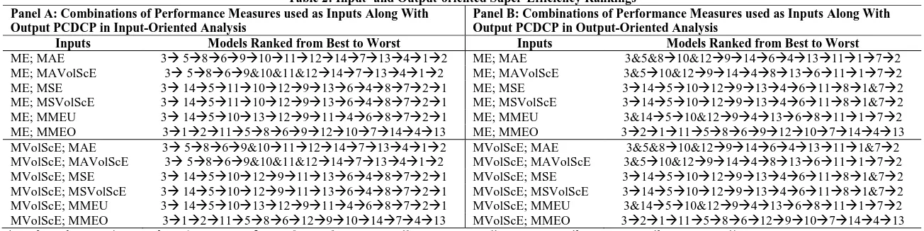
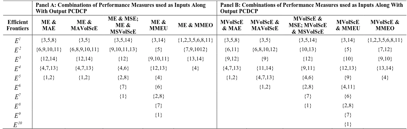
jJj1. Table 1 (respectively, Tables 2 and 4) provide the unidimensional (respectively, multidimensional) rankings of 14 forecasting models of crude oil prices’ volatility based on 9 measures of 3 criteria: biasedness, goodness-of-fit, and correct sign. Table 1 is a typical output presented by most existing forecasting studies – these unidimensional rankings are devised as follows: models are ranked from best to worst using the relevant measure of each of the criteria under consideration. Notice that different criteria led to different unidimensional rankings, which provides evidence of the problem resulting from the use of a unidimensional approach in a multicriteria setting. Table 2 summarizes multidimensional rankings, where the models are ranked from best to worst based on the corresponding super-efficiency scores obtained using both input-oriented and output-oriented radial super-efficiency DEA models. Notice that, under VRS conditions, the rankings of input- and output-oriented analyses are different and the rankings of output-oriented analysis show more ties. Table 3 provides the efficient frontiers obtained with SBM-CDEA. These results suggest that the best and the worst efficient frontiers are insensitive to adjusting biasedness measures for volatility. Note that any rankings based on these efficient frontiers would lead to a large number of ties. In order to break these ties, we use relative progress and attractiveness scoresobtained by solving models 3 and 4, respectively, which results in the multidimensional rankings provided in Table 4 where models are ranked from best to worst based on these relative scores. Notice that Tables 2 and 4 reveal that the multicriteria rankings of models obtained by input- and output-oriented super-efficiency DEA analyses and SBM-CDEA analysis are different. These differences are due to the fact that input-oriented analysis minimizes inputs for fixed amounts of output and output-oriented analysis maximizes outputs for fixed amounts of input, whereas orientation-free analysis optimizes both inputs and outputs simultaneously. In addition, oriented super-efficiency analyses only take account of technical efficiency, whereas orientation-free CDEA analysis takes account of an additional performance component; namely, slacks. In fact, for our data set – see Table 4, the efficient model SMA20 maintained its best position in the rankings regardless of the type of DEA analysis, because it is always on the best efficient frontier and has zero slacks regardless of the performance measures used. As to the rankings of the remaining models, there are differences that are mainly due to the presence of slacks and the nature of benchmarks.3 Inputs (respectively, outputs) consist of performance metrics to be minimized (respectively, maximized) according to the principle of the less
Table 1: Unidimensional Rankings of Competing Forecasting Models
Criteria Measures Ranked From Best to Worst
Biasedness Mean Error (ME) 3511914101241362871
Mean Volatility-Scaled Errors (MVolScE) 359&10&11&12&1446&132871
Goodness-of-fit
Mean Absolute Error (MAE) 85639&10111271413412 Mean Absolute Volatility-Scaled Errors (MAVolScE) 5&83&69&10&11&127&1413412 Mean Squared Error (MSE) 1413101211953648721 Mean Squared Volatility-Scaled Errors (MSVolScE) 14131011&12953648721 Mean Mixed Error Under-estimation penalized (MMEU) 1435101312911468721 Mean Mixed Error Over-estimation penalized (MMEO) 1278611129131014453 Correct Sign Percentage of correct direction change predictions (PCDCP) 3510&1291441368111&72
*1RW [Random Walk]; 2 HM [Historical Mean]; 3SMA20 [Simple Moving Average]; 4SMA60; 5SES [Single Exponential Smoothing]; 6ARMA(1, 1) [Auto Regressive Moving Average]; 7AR(1)
[AutoRegressive]; 8AR(5); 9GARCH(1, 1) [Generalized Auto Regressive Conditional Heteroscedasticity]; 10GARCH-M(1, 1); 11EGARCH (1,1) [Exponential GARCH]; 12TGARCH (1, 1) [Threshold
GARCH]; 13PARCH (1, 1) [Power Auto Regressive Conditional Heteroscedasticity]; 14CGARCH(1,1) [Component GARCH]
Table 2: Input- and Output-oriented Super-Efficiency Rankings Panel A: Combinations of Performance Measures used as Inputs Along With
Output PCDCP in Input-Oriented Analysis
Panel B: Combinations of Performance Measures used as Inputs Along With Output PCDCP in Output-Oriented Analysis
Inputs Models Ranked from Best to Worst Inputs Models Ranked from Best to Worst
ME; MAE 3 586910111214713412 ME; MAE 3&5&810&12914641311172 ME; MAVolScE 3 5869&10&11&1214713412 ME; MAVolScE 3&510&129144813611172 ME; MSE 3 145111012913648721 ME; MSE 31451012913461181&72 ME; MSVolScE 3 145111012913648721 ME; MSVolScE 31451012913461181&72 ME; MMEU 3 145101312911468721 ME; MMEU 3&14510&1294136811172 ME; MMEO 3121158691210714413 ME; MMEO 3211158691210714413 MVolScE; MAE 3 5869&10111214713412 MVolScE; MAE 3&5&810&129146413111&72 MVolScE; MAVolScE 3 5869&10&11&1214713412 MVolScE; MAVolScE 3&510&129144813611172 MVolScE; MSE 3 145101291113648721 MVolScE; MSE 31451012913461181&72 MVolScE; MSVolScE 3 145101291113648721 MVolScE; MSVolScE 31451012913461181&72 MVolScE; MMEU 3 145101312911468721 MVolScE; MMEU 3&14510&1294136811172 MVolScE; MMEO 3121158612910147413 MVolScE; MMEO 3211158612910714413
Table 3: Efficient Frontiers With Different Performance Levels Panel A: Combinations of Performance Measures used as Inputs Along
With Output PCDCP
Panel B: Combinations of Performance Measures used as Inputs Along With Output PCDCP
Efficient Frontiers
ME & MAE
ME & MAVolScE
ME & MSE; ME & MSVolScE
ME &
MMEU ME & MMEO
MVolScE & MAE
MVolScE & MAVolScE
MVolScE & MSE; MVolScE
& MSVolScE
MVolScE & MMEU
MVolScE & MMEO
1
E
{3,5,8} {3,5} {3,5,14} {3,14} {1,2,3,5,6,8,11} {3,5,8} {3,5} {3,5,14} {3,14} {1,2,3,5,6,8,11}2
E
{6,9,10,11} {6,8,9,10,11} {9,10,11,13} {5} {7,9,1012} {6,11} {6,8,10,12} {10,13} {5} {7,12}3
E
{12,14} {12,14} {12} {9,10,11} {13,14} {9,12} {9} {12} {10} {9,10}4
E
{4,7,13} {4,7,13} {4,6} {12,13} {4} {4,7,13} {11,14} {9,11} {12,13} {13,14}5
E
{1,2} {1,2} {2,8} {4} {1,2} {4,7,13} {4,6} {9} {4}6
E
{7} {6} {1,2} {2,8} {4,11}7
E
{1} {2,8} {7} {6}8
E
{7} {1} {2,8}9
E
{1} {7}10
E
{1}*1RW; 2 HM; 3SMA20; 4SMA60; 5SES; 6ARMA(1, 1); 7AR(1); 8AR(5); 9GARCH(1,1); 10GARCH-M(1,1); 11EGARCH(1,1); 12TGARCH(1,1); 13PARCH(1, 1); 14CGARCH(1,1)
Table 4: SBM-CDEA Rankings Panel A: Combinations of Performance Measures used as Inputs Along With
Output PCDCP
Panel B: Combinations of Performance Measures used as Inputs Along With Output PCDCP
Inputs Models Ranked from Best to Worst Inputs Models Ranked from Best to Worst
ME; MAE 3 5869&10111214134721 MVolScE; MAE 3 586109121411134721 ME; MAVolScE 3 511910681412413721 MVolScE; MAVolScE 3 510&126891411413721 ME; MSE 3 514911101312468271 MVolScE; MSE 3 514101312911468271 ME; MSVolScE 3 514911101312468271 MVolScE; MSVolScE 3 514101312911468271 ME; MMEU 3 145910111213468271 MVolScE; MMEU 3 145101213911468271 ME; MMEO 352111689,10&1214134 MVolScE; MMEO 3 52111681279&1014134
4. CONCLUSION
Xu and Ouenniche (2012a) proposed an input-oriented radial super-efficiency DEA-based framework to evaluate the performance of competing forecasting models of crude oil prices’ volatility, which delivers a single ranking based on multiple performance criteria; such a framework suffers from several issues that were overcome in this paper. The main results may be summarized as follows. First, models that are on the efficient frontier and have zero slacks regardless of the performance measures used (e.g., SMA20) maintain their ranks regardless of the choice of DEA analysis and its orientation. Second, the multicriteria rankings of the best and the worst models seem to be relatively robust to changes in most performance measures; in sum, SMA20 is the best across the board and, for the remaining models, differences in rankings were mainly due to the presence of slacks and the nature of benchmarks. Finally, when under-estimated forecasts are penalized, most GARCH types of models tend to perform well – suggesting that they often produce forecasts that are over-estimated. On the other hand, when over-estimated forecasts are penalized, averaging models such as RW, HM, SES tend to perform very well – suggesting that these models often produce forecasts that are under-estimated.
AUTHOR INFORMATION
Dr. Jamal Ouenniche is a Reader in Management Science at the University of Edinburgh, Business School, Edinburgh, UK. His research focuses on the design and implementation of mathematical programming-based and artificial intelligence-based methods. His papers have been published in journals such as Operation Research, European Journal of Operational Research, and International Journal of Production Research amongst others. E-mail: [email protected] (Corresponding author)
Dr. Bing Xu is a Lecturer at the School of Management & Languages; Accountancy, Economics and Finance; Heriot-Watt University; Edinburgh; EH14 4AS, UK. Her papers have been published in Expert Systems with Applications, Energy Economics, and Applied Financial Economics amongst others. E-mail: [email protected]
Professor Kaoru Tone is Professor Emeritus at the National Graduate Institute for Policy Studies, Tokyo, Japan. His papers have been published in European Journal of Operational Research, Journal of the Operational Research Society, Omega, International Transactions in Operational Research, and Annals of Operations Research amongst others.
REFERENCES
1. Banker, R. D., Cooper, W. W., Seiford, L. M., Thrall, R. M., & Zhu, J. (2004). Returns to scale in different DEA models. European Journal of Operational Research, 154, 345-362.
2. Majid, S.-D. (2012). On a basic definition of returns to scale. Operations Research Letters, 40, 144-147. 3. Morita, H., Hirokawa, K., & Zhu, J. (2005). A slack-based measure of efficiency in context-dependent data
envelopment analysis. Omega, 33, 357-362.
4. Seiford, L. M., & Zhu, J. (2003). Context-dependent data envelopment analysis – measuring attractiveness and progress. Omega, 31, 397-408.
5. Tone, K. (2001). A slacks-based measure of efficiency in data envelopment analysis. European Journal of Operational Research, 130, 498-509.
6. Xu, B., & Ouenniche, J. (2011). A multidimensional framework for performance evaluation of forecasting models: context-dependent DEA. Applied Financial Economics, 21, 1873-1890.
7. Xu, B., & Ouenniche, J. (2012a). A data envelopment analysis-based framework for the relative performance evaluation of competing crude oil prices’ volatility forecasting models. Energy Economics, 34, 576-583. 8. Xu, B., & Ouenniche, J. (2012b). Performance evaluation of competing forecasting models: A