Adaptive Control OF Nonlinear Multivariable
Dynamical Systems Using MRAN-RBF Neural
Networks
Tamer A. Al-zohairy
Computer Science Dept.Arriyadh Community Collage, Malaz, P.O Box 28095, Riyadh 11437, Saudi Arabia.
Abstract– Most practical systems have multiple inputs and multiple outputs, and the applicability of neural networks as practical adaptive identifiers and controllers will eventually be judged by their success in multivariable problems. In this paper, we design a model following adaptive controller for a class of a discrete time multivariable nonlinear systems. Radial Basis Function (RBF) neural network with Minimal Resource Allocation Network (MRAN) training algorithm is used for off-line stable identification. It implements a stable model following adaptive controller by utilizing the identification results. S imulation results demonstrate the proposed controller can drive unknown MIMO nonlinear systems to follow the desired trajectory very well.
Index Term − Adaptive control, MIMO systems, MRAN, RBF neural network, S equential learning algorithms.
I. INTRODUCTION
The success of model-based nonlinear control techniques is, usually, conditioned by the availability of highly reliable and accurate models which reflect most, if not all, of the nonlinear process complexities.
The most applied models in identification and control of the nonlinear systems are neural networks (NNs) and fuzzy logic systems (FLSs). The known supports of thes e models are their ability to learn and good performance for the approximation of the nonlinear functions. In the development of the neural networks, new structures are introduced everyday. New static and dynamic types of NNs are developed mostly to get better identification [1].
Most of the results reported in the literatures of the adaptive control of nonlinear dynamical systems are related to single-input single-output systems. Because most practical systems have multiple inputs and multiple outputs (MIMO), the efficacy of neural networks as practical adaptive controllers will eventually be judged by the applicability of the methodology developed so far to multivariable systems. Our interest in this paper is to study the problem of controlling a class of nonlinear multivariable systems whether they are known or unknown.
Radial Basis Function (RBF) neural networks have been popularly used in many applications in recent times due to their ability to approximate complex non -linear mapping directly from the input-output data with a simple topological structure and ease of implementation of dynamic and adaptive network architectures.
Several learning algorithms, such as resource allocation networks (RAN), RAN-EKF, and MRAN, have been proposed in the literature for training RBF networks. In practical on-line applications, sequential learning algorithms are generally preferred over batch learning algorithms as they do not require retraining whenever new data is received. However, selection of a learning algorithm for an on-line application is critically dependent on its accuracy and speed. In recent years, different methods [2]-[4] have been proposed in which sequential learning algorithms are used. Sequential learning algorithms have the following distinguishing features: 1) The input-output data are used sequentially
(one-by-one) to train the learning system;
2) At any sample time instant, only one input-output data can be observed and used by the learning system; 3) The learning system discards any observed input-output
data as soon as the learning procedure is completed; 4) The learning system has no prior knowledge as to how
many total training observations will be presented. A significant contribution to sequential learning was made by Platt [5] by proposing RAN in which hidden neurons were added sequentially based on the novelty of the new observed data. Enhancement of RAN, known as RAN-EKF, was proposed by [6] in which EKF rather than least mean squares (LMS) algorithm was used for updating the network parameters (centers, widths, and weights of Gaussian neurons) to improve the accuracy and obtain a more compact network. RAN and RAN-EKF can only add neurons to the network and can not prune insignificant neurons from the network. As a consequence, the networks obtained by RAN and RAN-EKF could become extremely large in some large-scale complex applications.
A significant improvement to RAN and RAN-EKF was made by [7], [8] by introducing a pruning strategy based on the relative contribution of each hidden neuron to the overall network output. The resulting network referred to as MRAN has been used in a number of applications [9]. Other pruning scheme in RBF networks have been proposed in [10], [11].
network output based on the input data distribution received in the window.
One important point to be noted in all of these sequential algorithms is that they do not link the required learning accuracy directly to the algorithm. Instead, they all have various thresholds which have to be selected using exhaustive trial and error studies. The issue of specifying various thresholds based on the needed accuracy has been raised in MRAN for determining the inactive neurons. In this paper, sequential learning algorithm MRAN [8] is used for identification and adaptive control of the MIMO nonlinear systems.
In this paper, we propose a method to design a model following adaptive controller for a class of a discrete time multivariable nonlinear systems. The structure of (MIMO) Radial Basis Function (RBF) Neural Network with sequential learning algorithm MRAN [8] is used for system identification and model following adaptive controller by utilizing the identification results. The simulation results demonstrate that the proposed control scheme can derive unknown MIMO systems to follow the desired trajectory very well.
This paper is organized as follows: In section II the problem and the plan of work are stated in detail. Section III gives details of control method for multivariable systems. In section IV MIMO Radial Basis Function (RBF) Neural Network is stated in detail. Section V gives a brief description of the MRAN learning algorithm. In section VI the structure of the overall adaptive system for off-line control using RBF is described. Section VII presents the simulation results on a real problem to prove the importance of the proposed model. Finally some conclusions are remarked in section VIII.
II. STATEM ENT OF THE PROBLEM
A discrete time nonlinear multivariable system be described by the difference equations:
∑
∑
∑
1 -L
0 j
n nj
n p n p 1
p 1 p n n
p
1 -L
0 j
2 j 2
n p n p 1
p 1 p 2 2
p
1 -L
0 j
1 j 1
n p n p 1
p 1 p 1 1
p
)j -k ( u b
)] 1 L -(k y , k), ( y , , ) 1 L -(k y , k), ( [y f 1) (k y
)j -k ( u b
)] 1 L -(k y , k), ( y , , ) 1 L -(k y , k), ( [y f 1) (k y
)j -k ( u b
)] 1 L -(k y , k), ( y , , ) 1 L -(k y , k), ( [y f 1) (k y
(1)
where, bij for (i:1n), (j:0L1), bi0 ≠0 are the
system parameters, u(k)[u1(k),u2(k),,un(k)]T and
T n p 2
p 1 p
p(k) [y (k),y (k), ,y (k)]
y are the input and
output vectors respectively, f1,f2,,fnare nonlinear
functions, and Ln.
Consider the linear reference model described by the second-order difference equations of the form:
) 1 -k ( r b ) k ( r b
) 1 -k ( y a -) k ( y -a ) 1 k ( y
) 1 -k ( r b ) k ( r b
) 1 -k ( y a -) k ( y -a ) 1 k ( y
) 1 -k ( r b ) k ( r b
) 1 -k ( y a -) k ( y -a ) 1 k ( y
n n1 m n
n0 m
n m n2 m n m n1 m n
m
2 21 m 2
20 m
2 m 22 m 2 m 21 m 2
m
1 11 m 1 10 m
1 m 12 m 1 m 11 m 1
m
(2)
where ym(k)[ym1,ym2,,ymn]T and r(k)[r1(k), (k)]
r , (k),
r2 n are the model output and bounded
reference input vectors respectively and
i1 m i0 m i2 m i1
m ,a ,b ,b
a for (i:1n) are known
parameters.
The control problem is to determine the bounded input vector u(k)[u1(k),u2(k),,un(k)]T so that the plant output vector yp(k)[yp1(k),yp2(k),,ypn(k)]T
follows the model output vector
, y , y [ ) k (
ym m1 m2
T n m ]
y ,
asymptotically, that is,
0 ) k ( y -) k ( y
limk pi mi for(i:1n).
Our objective here is to develop a new method to design a model following adaptive controller for discrete time multivariable nonlinear systems given in (1) using MIMO Radial Basis Function (RBF) Neural Network with sequential learning algorithm MRAN.
We shall consider the cases where
1) The functions f1,f2,,fn and the parameters
ij
b (i:1n), (j:0L1) are known.
2) The functions f1,f2,,fn and the parameters
ij
b (i:1n), (j:0L1) are unknown.
The first problem is one of nonlinear control. The second problem is about adaptive control. If a solution to problem 1) exists, our next objective is to find it adaptively for problem 2) where f1,f2,,fnand bij(i:1n),
) 1 L 0 : j
( are unknown.
III. MIM O SYSTEM CONTROLLER
In this section we consider the problem of controllin g the plant described in section II. As we will see, if the functions f1,f2,,fn in (1) are known, it follows directly that at stage k, u(k)[u1(k),u2(k),,un(k)]Tcan be
computed from the knowledge of
T n p 2
p 1 p
p(k) [y (k),y (k), ,y (k)]
y and its past values.
Let the difference equations of a plant be given by (1). Let a reference model is described by the second order
difference equations given by (2) where
T n 2
1(k),r (k), ,r (k)]
r [ ) k (
r represent a bounded
) k ( y ) k ( y ) k ( y ) k ( y ) k ( y ) k ( y ) k ( e ) k ( e ) k ( e pn 2 p 1 p mn 2 m 1 m n 2 1
(3)
the aim of control is to determine a bounded control input
) k (
u such that
0 ) k ( e
limk . (4)
Now, let us assume that at the steady state the following condition is satisfied:
) k ( e ) k ( e ) k ( e ) 1 k ( e ) 1 k ( e ) 1 k ( e n 2 1 n 2 1
(5)
From (5), the following equation is obtained:
) k ( y ) k ( y ) k ( y ) k ( y ) k ( y ) k ( y ) 1 k ( y ) 1 k ( y ) 1 k ( y ) 1 k ( y ) 1 k ( y ) 1 k ( y pn 2 p 1 p mn 2 m 1 m pn 2 p 1 p mn 2 m 1 m
(6)
By substituting from (1) and (2) into (6) and replacing
) k (
ymi with ypi(k) for (i:1n), we obtain
) 1 j k ( u b )] L k ( y , ), 1 k ( y , ), 1 L k ( y , ), k ( y [ f ) k ( y ) j k ( u b )] 1 L k ( y , ), k ( y , ), 1 L k ( y , ), k ( y [ f ) 1 k ( r b ) k ( r b ) 1 k ( y a ) k ( y a 1 L 0 j i ij pn pn 1 p 1 p i pi i 1 L 0 j ij pn pn 1 p 1 p i i 1 mi i 0 mi pi 2 mi pi 1 mi
(7)Notice that the first term ymi(k) on the right hand side
in (6) is not replaced with (2). From (7) the plant input
) k (
ui for(i:1n) can be computed from the knowledge
of ypi(k) and its past values as
1 L 1 j 1 L 1 j i ij i ij i 0 i pn pn p1 1 p i pn pn p1 1 p i i 1 mi i 0 mi pi 2 mi pi 1 mi 0 i i )}. 1 j k ( u b ) j k ( u b ) 1 k ( u b )] L k ( y , ), 1 k ( y , ), L k ( y , ), 1 k ( y [ f )] 1 L k ( y , ), k ( y , ), 1 L k ( y , ), k ( y [ f ) 1 k ( r b ) k ( r b ) 1 k ( y a ) k ( y ) 1 a ( { b 1 ) k ( u (8)Substituting (8) into (1), we obtain
) 1 k ( r b ) k ( r b ) 1 k ( y a ) k ( y a ) 1 k ( y i 1 mi i 0 mi pi 2 mi pi 1 mi pi (9)
Then, the error ei(k1) is given by
) 1 k ( e a ) k ( e a 1)) -(k y 1) -(k (y a (k)) y (k) (y a ) 1 k ( y ) 1 k ( y ) 1 k ( e i 2 mi i 1 mi pi mi 2 mi pi mi 1 mi pi mi i (10)
Therefore, the following condition is satisfied for arbitrary initial value ei(0):
0 ) k ( e
limk i (11)
IV. RADIAL BASIS FUNCTION NETWORK (RBFN) In case of MIMO system given by (1), the RBF network with multiple outputs is appropriate for identification problem. Fig. 1 shows a typical RBF network, with q inputs (x1,, xq), and p outputs
) y , , y
( 1 p . The hidden layer consists of h computing units connected to the output by h weight vectors
) , ,
(1 h . The response of one hidden unit to the network input at the ith instant, xi, can be expressed by
i 2
k i 2 i k i k x ) ( 2 1 exp ) x
( , (k :1h) (12)
where i
k
is the center vector for kth hidden unit at ith
instant, ik is the width of the Gaussian function at that time, and . denotes the Euclidean norm. The overall network response is given by
h 1 k i k i k i 0 ii f(x ) (x )
yˆ (13)
where p
i R
y , xiRq. The coefficient vector ik is the connecting weight vector of the kth hidden unit to output
layer, which is in the vector form of
i
pk i lk i k 1 i
k , , , ,
. Thus the coefficient matrix
of the network can be expressed as
i ph i pk i 1 p i lh i lk i 1 l i h 1 i k 1 i 11 i h p A
and the bias vector is
ip0
i 0 l i 10 i
0 , , , ,
.
V. TRAINING RBFN USING MRAN ALGORITHM Learning of MRAN begins with no hidden units, that is h0. As input-output training data (x ,y)
i
i is received,
a) Allocation of a new hidden unit.
This first step of the algorithm is to check whether following three conditions are satisfied:
min i
i
i y f(x ) e
e (14)
i i nr i
x (15)
min w
i
) 1 n ( i j
2 j T j i
rms e
n e e
e w
(16)
Where i
nr
is the center of the hidden unit which is closest to xi. emin, i and emin are thresholds to be selected appropriately. emin used to determine if the existing nodes are insufficient to obtain a network output is an instantaneous error check. i ensures that the new neuron is sufficiently far from all the existing neurons and is given by imax
max,min
where is decay constant) 1 0
( . Equation (16) is introduced to ensure the neuron growth is smooth. ej is the network output error at jth
instant and emin is the threshold selected to check whether the network meets the required sum squared error specification over a sliding window of size nw in the past. If the three error criteria in (14), (15), (16) are satisfied, a new hidden neuron is added to the network with the following initial parameters to remove error:
i nr i i
1 h
i i
1 h
i i
1 h
x x e
(17)
where is an overlap factor which determines the overlap of the hidden neurons responses with the neighbor hidden units in the input space. After the new hidden unit is allocated, go to (c) to prune redundant hidden units.
b) Updating the parameters using Extended Kalman Filter
(EKF)
In this step, the network parameters
T i h T i h T i h i 1 T i 1 T i 1 T i 0 ) 1 Z (
i [ , , , , , , , ]
W (18)
are adapted using original EKF. The posterior parameter estimate is calculated from its prior estimate Wi, Kalman gain Ki and error eias follows:
1) (p i p) (z i 1) (z 1 i 1) (z
i W K e
W (19)
The Kalman gain can be calculated as:
1 i 1 i T i ) p p ( i p) (z i z) (z 1 i p) (z
i P B [R B P B ]
K (20)
where Bi is the gradient matrix given by
) x ( f
Bi Wi1 i (21)
and Pi is the error covariance matrix, which is updated by
z) (z 1 i T i i z) (z
i [I KB ]P qI
P (22)
Where q is a coefficient that determines the allowed random step in the direction of the gradien t matrix. This term qI causes that avoidance of local minimum.
Moreover, when the new hidden unit is allocated in (b), the dimensionality of Pi is increased by
1 1 z z 0 1 i i 0 p I
0 P
P (23)
where the new rows and columns are initialized by p0. p0 is an estimate of the uncertainty when the initial values assigned to the parameters. The dimension z1 of the identity matrix I is equal to the number of new parameters introduced by the new hidden neurons. Then go to (c) to prune redundant hidden units.
c) Pruning Strategy
The last step of the algorithm is to prune redundant hidden units that have little contribution to the network outputs for
w
n consecutive observations in the sliding data window. To accomplish this objective, the contribution of all the available hidden units (k:1h) are first calculated on the network outputs (l:1p) as follows:
) x (
Oikl iklk i (24) The highest absolute values of these contribution values are:
T i kp k i
1 k k i i
max(x) [maxO , ,maxO ]
O (25)
Now, the contribution values on each network output are normalized to the highest absolute values as follows:
i max
i kl i
kl
l
O O
r ; (k:1h) (l:1p) (26)
If the normalized contribution value of the kth hidden unit on the lth network output rkl falls below a threshold for
w
n consecutive observations, the kth hidden unit is regarded as a redundant unit and is pruned. Then the dimensionality of the covariance matrix Pi in the EKF learning algorithm is adjusted by removing rows and columns which are related to the pruned unit.
VI. RBFN CONTROLLER DESIGN FOR MIM O NONLINEAR SYSTEM
1) The functions f1,f2,,fn and the parameters
ij
b (i:1n), (j:0L1) are known.
2) The functions f1,f2,,fn and the parameters
ij
b (i:1n), (j:0L1) are unknown.
The various steps involved in the design of identifiers and controllers are described in detail.
A. The Functions f1 ,f2 , ,fnand the Parameters bij are Known
If the functions f1,f2,,fnand the parameters bij for
) n 1 : i
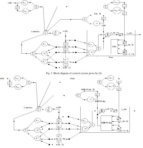
( , (j:0L1) are known the controller is given by (8). In this case RBFN is not used. The structure of the overall control system is shown in Fig. 2. Where
L k ( y , ), k ( y , ), 1 L k ( y , ), k ( y [ f ] k [
fi i p1 p1 pn pn
)] 1
for (i:1n) and biT [bi1 bi2 bi(L-1)].
B. The Functions f1 ,f2 , ,fnand the Parameters bij are Unk nown
Because our interest is primarily in adaptive control, nonlinear functions f1,f2,,fnand parameters bij for
) n 1 : i
( , (j:0L1), bi0 ≠0 are assumed to be
unknown. A three stage procedure is usually employed to determine a nonlinear controller that performs satisfactorily. The three stages will be discussed in the following subsections.
1) Identification of the functions f1 ,f2 , ,fn
It is clear that when nonlinear functions f1,f2,,fn are unknown the input-output data required to construct a single MIMO RBF neural network must be generated from the actual nonlinear functions f1,f2,,fn. This is commonly achieved by the application of random inputs
)] 1 L -(k y , k), ( y , , ) 1 L -(k y , k), ( [y
k p1 p1 pn pn
in a suitably chosen range and by adjusting the parameters
T i h T i h T i h i 1 T i 1 T i 1 T i 0 ) 1 Z (
i [ , , , , , , , ]
W of the RBF
network using the nonlinear system functions input-output to minimize the identification error. The fact that the output of the nonlinear system functions can be measured permits the use of one MIMO RBF neural network given in section IV with the MRAN training algorithm given in section V to identify nonlinear functions f1,f2,,fn. Further, for the procedure to be valid, the system functions must be assumed to be bounded-input bounded-output stable for the class of inputs used. The RBF neural network model generated in such manner is adequate for accurate control.
2) Identification the unk nown parameters bij
If the output of the nonlinear system ypi(k1) for )
n 1 : i
( and output of the functions f1,f2,,fn can be measured, the system given by (1) can be represented as
n T n n n
p
2 T 2 2 2
p
1 T 1 1 1
p
b u ] [k f -1) (k y
b u ] [k f -1) (k y
b u ] [k f -1) (k y
(27)
Where u [ui(k) ui(k 1) ui(k-L 1)]
T
i and
] b b b [
biT i1 i2 i(L-1) .
The unknown vectors b1,b2,,bn can be obtained by applying the conventional recursive least-squares method as follows:
) 1 k ( u ) 1 k ( P ) 1 k ( u ) k (
) 1 k ( P ) 1 k ( u ) 1 k ( u ) 1 k ( P ) 1 k ( P ) k (
1 ) k ( P
) 1 k ( u ) 1 k ( P ) 1 k ( u ) k (
) 1 k ( u ) 1 k ( P )
k (
) 1 k ( bˆ ) 1 k ( u ) k ( y ) k ( e
) k ( e ) k ( ) 1 k ( bˆ ) k ( bˆ
i T
i
T i i
i T
i
i i T
i pi
i i
(28) 3) Offline Controller Design
In this stage, the identifier (single MIMO RBF) of the nonlinear functions f1,f2,,fn described in section VI. B. 1 and the system parameters bij for (i:1n), (j:0L1)
obtained in section IV. B. 2 by applying the conventional recursive least-squares method are used for off-line control. The structure of the overall adaptive system is shown in Fig. 3. Where the functionfi in Fig. 2 is replaced by the ithoutput of the MIMO RBFN, RBFNi, and the system parameters bijtakes the values obtained from applying recursive least-squares method.
VII. SIM ULATION RESULTS
In this section, the performance of the proposed controller is demonstrated through simulation resu lts. Two MIMO nonlinear plants with two inputs and two outputs widely used as benchmark examples [12]-[13] have been taken for this purpose.
Example 1 [12]:
Consider a MIMO system described by the following equation:
) k ( u b
) k ( u b )] k ( y ), k ( y [ f
)] k ( y ), k ( y [ f ) 1 k ( y
) 1 k ( y
2 20
1 10 p2
1 p 2
p2 1 p 1 2
p 1 p
(29)
where
1 b
1 b
20 10
(30)
) k ( y 1
) k ( y ) k ( y )] k ( y ), k ( y [ f
y 1
) k ( y )] k ( y ), k ( y [ f
2 2 p
2 p 1 p p2 1 p 2
2 p 1 p p2
1 p 1
(31)
On the other hand, the reference model is given by
) k ( r 1 . 0
) k ( r 3 . 0 ) k ( y
) k ( y 0.6 0.1
0.2 3 . 0 ) 1 k ( y
) 1 k ( y
2 1 2
m 1 m 2
m 1 m
(32)
Where the external inputs have the form
25 k 2 cos
25 k 2 sin
) k ( r
) k ( r
2
1 (33)
Because the output of nonlinear system functions
2 1 ,f
f can be measured we can use one MIMO RBF neural network given in section IV with the MRAN training algorithm given in section V to identify nonlinear functions f1 ,f2. The parameters for the MRAN used here are: max4.0, min 0.9, 0.98,emin 0.09,
1 . 0
emin , 0.8, P01.0, Ri1, q0.004, nw80, 00001
. 0
. The identification procedure was carried out with random inputs u1(k) and u2(k) uniformly
distributed in the interval[1,1].
The unknown system parameters b10,b20 can be obtained by applying the conventional recursive least -squares method given in section IV. B. 2. After applying the conventional recursive least-squares method, values of
20 10,b
b have the same values as that of the actual system given by (30).
After the MIMO plant is identified and the unknown system parameters b10,b20 were obtained, the control process is initiated using the adaptive system shown in Fig. 3. Fig. 4 shows that the tracking performance is satisfactory and the RMS error is 0.05. Fig. 5 shows the control input resulting from the control structure given by Fig. 3.
Example 2 [13]:
The MIMO plant considered here is described by the following equation:
) k ( u
) k ( u
) k ( y 1
) k ( y ) k ( y
) k ( y 1
) k ( y
) 1 k ( y
) 1 k ( y
2 1
2 2 p
p2 1 p
2 2 p 1 p
2 p
1 p
(34)
where
1 b
1 b
20 10
(35)
-0.6 -0.4 -0.2 0 0.2 0.4 0.6
0 10 20 30 40 50 60 70 80 90 100
k
y
m
1
&
y
p
1
-0.25 -0.2 -0.15 -0.1 -0.05 0 0.05 0.1 0.15 0.2 0.25
0 10 20 30 40 50 60 70 80 90 100
k
y
m
2
&
y
p
2
Error! Not a valid link.Fig. 4. Example 1: Performance of the controller given by Fig. 3 when RBF neural network is used; solid line is the desired output of the plant, and dashed line is the actual output.
-0.2 -0.15 -0.1 -0.05 0 0.05 0.1 0.15 0.2
0 10 20 30 40 50 60 70 80 90 100
k
u
1
-0.3 -0.25 -0.2 -0.15 -0.1 -0.05 0 0.05 0.1 0.15 0.2 0.25
0 10 20 30 40 50 60 70 80 90 100
k
u
2
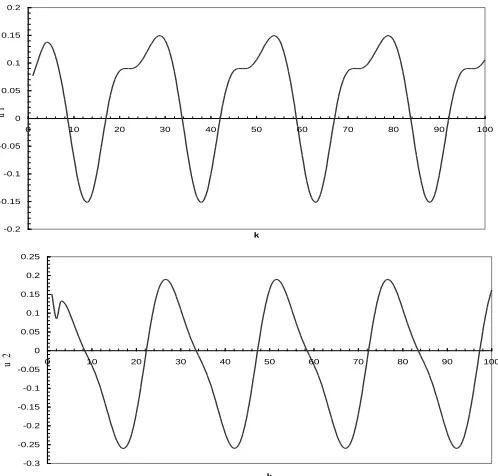
Fig. 5. Example 1: The requested control signals using the controller based RBF neural network given by Fig. 3.
and
) k ( y 1
) k ( y ) k ( y )] k ( y ), k ( y [ f
y 1
) k ( y )] k ( y ), k ( y [ f
2 2 p
2 p 1 p p2
1 p 2
2 2 p 1 p p2
1 p 1
(36)
random inputs u1(k) and u2(k) uniformly distributed in
the interval[1,1].
If the parameters b10,b20 of the system (34) are unknown. The conventional recursive least-squares method given in section IV. B. 2 can be used to obtain them. After applying the conventional recursive least-squares method, values of b10,b20 have the same values as that of the actual system given by (35).
The control of the nonlinear multivariable model of plant given by (34) is carried out using the adaptive system shown in Fig. 3.
The performance of the proposed method for controlling was tested with the reference model given by
) k ( r
) k ( r 0.8 0.1
0.2 6 . 0 ) 1 k ( y
) 1 k ( y
2 1 2
m 1 m
(37)
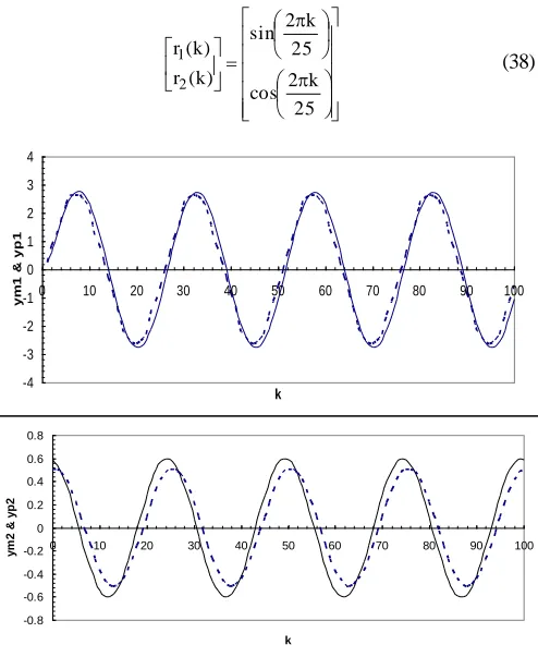
is shown in Fig. 6, and the control signals are shown in Fig. 7, where the external inputs taken have the form
25 k 2 cos
25 k 2 sin
) k ( r
) k ( r
2 1
(38)
-4 -3 -2 -1 0 1 2 3 4
0 10 20 30 40 50 60 70 80 90 100
k
ym
1
&
yp
1
-0.8 -0.6 -0.4 -0.2 0 0.2 0.4 0.6 0.8
0 10 20 30 40 50 60 70 80 90 100
k
ym
2
&
yp
2
Fig. 6. Example 2: Performance of the controller given by Fig. 3 when RBF neural network is used; solid line is the desired output of the plant,
and dashed line is the actual output.
-1 -0.8 -0.6 -0.4 -0.2 0 0.2 0.4 0.6 0.8 1
0 10 20 30 40 50 60 70 80 90 100
k
u
1
-1 -0.5 0 0.5 1 1.5 2
0 10 20 30 40 50 60 70 80 90 100
k
u
2
Fig. 7. Example 2: T he requested control signals using the controller based RBF neural network given by Fig. 3.
VIII. COM PARISON WITH OTHER WORK In this section, we will make a comparison between the method given above to obtain controller using RBF neural network with the MRAN training algorithm and that given in [12] and [13] to control the same system using recurrent neural networks.
From the results obtained above and that in [12] and [13] to solve the same problem it was found that:
1) Recurrent network used in [12] and [13] for control is quite slow and computationally intensive compared to that proposed in this paper using RBF model with MRAN algorithm to solve the same problem.
2) The performance given in both may be the same but the control method proposed in this paper is faster than that used in [12] and [13] to solve the same problem which makes our proposed method more suitable for real time problems.
IX. CONCLUSION
In this paper, we have proposed a new model following adaptive controller for a class of a discrete time multivariable nonlinear systems. In the proposed method, Radial Basis Function (RBF) neural network with Minimal Resource Allocation Network (MRAN) training algorithm were used for off-line stable identification and implements a stable model following adaptive controller by utilizing the identification results. Simulation results and a comparison study have revealed that the proposed control method is suitable for a class of discrete time multivariable nonlinear systems. The general conclusion, therefore, is that RBFN should be preferred to the recurrent network in control problems because it requires less training time to converge and fewer computational complexities to train the network.
ACKNOWLEDGEM ENT
The author would like to thank King Saud University for its academic support throughout the research work.
REFERENCES
[1] Madan M. Gupta, Liang Jin, Noriyasu Homma, “Static and Dynamic neural Networks From Fundamentals to Advanced T heory,” John Wiley&Sons Inc., 2003.[14]
[2] Huang G. B., et al., "A Generalized Growing and Prunin g
RBF (GGAP -RBF) Neural Network for Function
Approximation," IEEE Trans. Neural Networks, Vol. 16, No. 1, 2005.
[3] Julier S. J. and Uhlmann J. K., “A New Extension of the Kalman Filter to Non-Linear Systems,” in: Proc. Of AeroSense: T he 11th Int. Symp. A.D.S.S.C., 1997.
Networks,” SICE Annual Conference in Sapporo, August, 2004.
[5] Platt J., “A Resource-Allocating Network for Function Interpolation,” Neural Computat., Vol. 3, pp. 213-225, 1991. [6] Kadirkamanathan V. and Niranjan M., “A Function Estimation Approach to Sequential Learning with Neural Networks,” Neural Computat., Vol. 5, pp. 954 – 975, 1993.
[7] Yingwei L., et al., “A Sequential Learning Scheme for Function Approximation Using Minimal Radial Basis Function (RBF) Neural Networks,” Neural Computation, Vol. 9, pp. 461-478, 1997.
[8] Yingwei L., et al., “Performance Evaluation of a Sequential Minimal Radial Basis Function (RBF) Neural Network Learning Algorithm,” IEE T rans. Neural Networks, Vol. 9, No. 2, pp. 308-318, 1998.
[9] Sundararajan N., et al., “Radial Basis Function Neural Networks with Sequential Learning: MRAN and its Applications,” Rever Edge: Singapore; World Scientific: NJ, 1999.
[10] Rojas I., et al., “ Time Series Analysis Using Normalized PG-RBF Network with Regression Weights,” Neurocomputing, Vol. 42, pp. 267-285, 2002.
[11] Salmer'on M., et al., “Improved Ran Sequential Prediction Using Orthogonal echniques,” Neurocomputing, Vol. 41, pp. 153-172, 2001.
[12] Li Y., Powers D., and Wen P., “Internal Model Control Using Recurrent Neural Networks For Nonlinear Dynamical Systems,” Proceeding of the International Conference on Artificial Intelligence, 2001.
[13] K. S. Narendra and K. Parthasarathy, “Identification and control of dynamical systems using neural networks,” IEEE T rans. Neural Networks, vol. 1, pp. 4 -27, Mar. 1990.
Tame r A. Alz ohairy received the B. Sc. Degree in computer science from faculty of Science, Ain Shams University, Cairo, Egypt in 1989. M.Sc degree in Computer science from Math. Dept., Faculty of science, Al-Menoufia university, Egypt, in 1997 and Ph.D in computer science from math. Dept. Faculty of science, Suez Canal University, Egypt in 2003. He is working currently in Computer science Dept., Community college, King Saud University. Saudi Arabia on leave from Math. Dept., faculty of science, Al-Azhar university, Cairo, Egypt .
Fig. 2. Block diagram of control system given by (8).