Warp-Knitted Fabrics Simulation Using Cardinal Spline and Recursive Rotation Frame

Warp-Knitted Fabrics Simulation Using Cardinal

Spline and Recursive Rotation Frame

Aijun Zhang1, Xinxin Li1, Sha Sha1, Gaoming Jiang1,2

1

Engineering Research Center for Knitting Technology, Jiangnan University, Wuxi, Jiangsu CHINA

2

International Joint Research Laboratory for Noval Knitting Structural Materials, Jiangnan University, Wuxi, Jiangsu CHINA

Correspondence to:

Aijun Zhang email: [email protected]

ABSTRACT

To realize 3-D simulation of warp-knitted fabrics, this paper proposes a 3-D loop modeling method based on Cardinal spline and recursive rotation frame method. Fabric structure and loop geometry are studied to form a visible lapping detection model and loop geometrical key points obtained according to chain links and yarn arrangements. In this paper, eight points are set for stitched loop and three points for the inlay. To connect all the control points via a curved line to form a knitted loop shape, the Cardinal spline method is adopted because it is simple to calculate and adjustable in radians. A recursive rotation frame is established to calculate the coordinates of the yarn cross section, eliminating the problem of yarn discontinuity caused by excessive rotation of the moving frame. With the 3-D loop modeling method, some specific mesh and spacer structures are simulated to demonstrate applicability.

INTRODUCTION

Warp-knitted fabrics, with comparatively complicated structures, are comprised of overlaps and underlaps. Overlaps are looped in the longitudinal direction to form wales while underlaps connect wales in transverse direction. Various overlaps and underlaps are formed when different lapping movements are made by guide needle bars. Yarn coverage is caused as several guide needle bars overlap and underlap at the same time, which additionally adds more complexity challenges warp-knitted fabrics designers. With the wide application of computer graphics technology in textiles, computer-aided simulation of warp-knitted fabrics, especially in three-dimensional structures, has become increasingly important.

Much research has been done on 3-D simulation of fabrics and yarn modeling, which normally consists of the following two steps: building a yarn path curve according to the fabric structure geometry followed by formation of a 3-D model based on the sectional features of the yarn.

splines such as the natural cubic spline and Catmull-Rom spline methods account for all of the control points, and thus are more appropriate for determining the yarn path of warp-knitted fabrics.

After the yarn path curves are drawn, a 3-D yarn model is usually built by sweeping along the path curve with a section plane or sphere due pipe-like shape of the yarn. Li [10] created weft-knitted yarn model of fixed diameter by sweeping the path with a sphere; Sherburn [7] simulated yarns of various section shapes by changing the section functions in woven fabrics; Durville [14] simulated the fiber structure of woven fabrics and Goktepe [13] simulated warp-knitted fabrics with a sweeping algorithm.

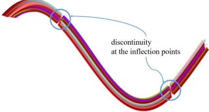
In sweep-based geometrical modeling, a basic problem is the determination of the local moving frame, especially for the case where the path is a spatial curve which directly affects the shape control of the generated sweep surface. Frenet frames and Rotation Minimizing frames [15] are mostly used in Computer Graphics. Each coordinate direction of the Frenet frame has a clear geometric meaning and basic formula. However, the Frenet frame has discontinuous frames at the inflection point, and it is difficult to control the twist of the local frame. These defects produce phenomena similar to Figure 1 [16]. The Rotation Minimizing Frame overcomes these disadvantages but does not solve the equation explicitly. Liao [17] preferred the Frenet frame method when simulating tubular braided fabric; Goktepe [13] chose the Gram-Schmidt algorithm to obtain an orthogonal vector group as the local frame; Adanur [18] set one vector parallel to the z axis to simplify the computation; Sherburn [7] redefined the vector parallel to the z axis to avoid the condition that the denominator equals zero. Nevertheless, the method of fixing one vector of the frame is more suitable for woven fabrics than warp-knitted fabrics because warp-knitted fabrics feature complex interloops in 3-D space while the yarn path of woven fabrics can be regarded as a planar curve.

FIGURE 1. Discontinuous yarns when simulated.

To simulate warp-knitted fabrics, this paper chooses a simple but efficient Cardinal spline method to draw the yarn path curve and adopts a recursive rotation frame method to solve the section coordinates of the yarn and form a 3-D yarn surface.

GEOMETRICAL LOOP STRUCTURE

A spline curve is defined by the control points. Renkens [19], Zhang [12] and Goktepe [20] all determined control points suitable for their spline models. This section describes the determination of the control points suitable for the Cardinal spline.

Spatial Structure

(a)

(b)

FIGURE 2. Warp-knitted structures: (a) stitched loop structure; (b) inlay structure.

Figure 3-a shows a side view of a two-guide-bar loop structure, which is divided into six layers from the technical back to the technical face. Underlaps occur on layer 1 and layer 2; overlaps occur on layer 3 and layer 4; loop arms occur on layer 5 and layer 6. The second bar (Figure 3-b) shows an inlay structure. The side view is divided into 4 layers with no overlap and loop arms for the inlay guide bar. Likewise, a side view of a multiple-guide-bar structure has tripled layers- the front bar underlaps and overlaps are respectively located on the left and right layers while the back bar underlaps and overlaps are located on the middle layers.

(a) (b)

FIGURE 3. Warp-knitted structures: (a) Side view of stitched loop

Based on the above statement, for multiple-guide-bar structure, each warp yarn layer division is inferred from the following equations:

ui =

L i (1)

oi = + + −1

L T S i (2)

2 1

= + × + −

ai

L T S i (3)

Where Lui is the layer of underlap of bar No. i; Loi is

the layer of overlap of bar No. i; Lai is the layer of

loop arms of bar No. i; T is the total number of guide bars and S is total of bars for stitching.

Structural Control Points

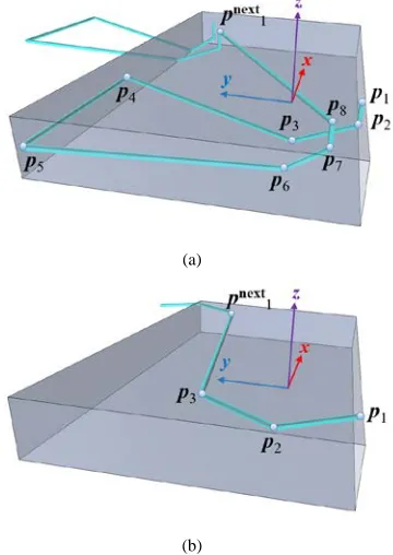
3-D loop structures are drawn using the spline curve method after obtaining the structural control points. The number of control points greatly affects the spatial structure of loops. If excessive control points are used, the smoothness of loop curve is reduced. If too few control points are used, it’s impossible to form a complete loop shape. With reference to Dabiryan's method [2], this paper proposes a 3-D loop model with 8 control points for stitched loop structures and 3 control points for inlay structures after the loop are accounted for, as shown in Figure 4.

(a)

(b)

Figure 4-a depicts a stitched loop structure consisting of four segments: the overlap (p4p5), two arms (p2p3p4, p7p6p5), two roots (p1p2, p8p7) and the underlap (p8pnext1). The loop coordinates are located in the middle of p3 and p6. The position of each point pk = (xk, yk, zk) can be calculated according to Table I.

TABLE I. Control points of stitched loop.

Point x y z

p1

∑

i t t

c d −2.5×dmax

-1 ( ) 1

2 =

− i−

∑

d d

p2

∑

i t t

c d −2.5×dmax

-1 ( ) 1

2 =

− i−

∑

d d

p3

∑

i t t

c d ₀ -1 _{( )}

1

2 =

− i−

∑

h −₂−

∑

oi L i t l l d d p5 2 ×

−c w h −₂−

∑

oi L i t l l d d

p6 − ∑=₁

i t t

c d 0 −₂−

∑

ai L i t l l d d

p7 − ∑₌₁

i t t

c d −1.5×dmax

-1 ( ) 1

2 =

− i−

∑

d d

p8 − ∑=1

i t t

c d −1.5×dmax

-1 ( ) 1

2 =

− i−

∑

d d

In Table I,i is the guide needle bar number; dt is the

diameter of yarn in bar number t; dmax is the

maximum diameter of all yarns; t(l) is the bar number of layer l; h is height of the loop; w is width of the loop, namely the distance between p4 and p5; c is the lapping mode of stitched loop. If c=1, the guide needle bar overlaps from right to left; if c=-1, the guide needle bar overlaps from left to right.

As shown in Figure 4-b，the inlay structure consists of two sections: inlay arc (p1p2p3) and underlap (p3pnext1). The loop coordinates are located in same position as in the loop mentioned above; the position of each point is derived from the equations in Table II, where c' is the lapping mode of the inlay. If c'=1, the control points are located right of loop; if c'=-1, the control points are located left of loop.

TABLE II. Control points of inlay structure.

Point x y z

p1 '

5

×w

c −0.4×h −₂−

∑

ui L i t t d d

p2 '

2

×w

c 0 −₂−

∑

ui L i t t d d

p3 '

5

×w

c 0.4×h −₂−

∑

When the yarns pass through a loop, it is theoretically possible that front bar yarns stay in the middle and back bar yarns stay aside, but in actuality their position is affected by the chain links. The initial control point position has to be adjusted. In Figure 5-a, p1 and p'1 are respectively the underlap inlets of front bar and back bar, while p8 and p'8 are respectively the underlap outlets of front bar and back bar. When the yarns are loaded with force, shifts of underlap inlets and outlets will occur. Relative positions of p8 and p'8 are free to change, but restricted for p1 and p'1. Control points of underlaps are modified by the following steps:

(a) (b) (c)

FIGURE 5. Control points of underlap. (a) initialized control points; (b) points position when loaded with force; (c) the modified control points.

i. The underlap inlets remain the initialized ones while the outlets change in reference to the outlet direction, shown as Figure 5-b;

ii. Relative positions of underlap inlets and outlets should be checked according to the lapping mode. If c=1, the underlap inlet of front bar should remain to the right, shown as Figure 5-c.

LOOP DEFORMATION BEHAVIOR

(a) (b)

FIGURE 6. Loops in initialized and deformed conditions. (a) loops in initialized condition; (b) loops in deformed condition.

3-D LOOP MODELING

Key control points of loop and inlay are achieved according to the statement above. When achieved, the control points are connected by line segments to form the basic frame of loops. However, the loop line segments must be modified based on non-rigid features. Therefore, this paper uses a popular approach to build loop models in which control points of loops knitted by one yarn are solved first (shown in Figure 7-a) and then connected by continual curves with Cardinal spline method (shown in Figure 7-b). Afterwards, loop model surface is created by defining a section curve and sweeping along the yarn path line (shown in Figure 7-c).

(a)

(b)

(c)

FIGURE 7. 3-D yarn drawing process. (a) control points of yarn; (b) yarn path curve and section curves; (c) loop model with twisted

Yarn Path Curve

Cardinal spline, a curve of segmental cubic polynomial interpolation [24], is used to form loop model surfaces for the following reasons: first, the Cardinal spline goes through all of the control points; second, only four neighborhood segmental lines are changed when one control point is moved; finally, the tensor of each segmental line is individually defined. Cardinal spline is solved according to the following equation:

( )

1

1 2

1

1 3 3 1

2 2 2 2

5 1

1 2

2 2

1 1

0 0

2 2

0 1 0 0

−

+ +

 

=  

− + + − − −

 

 

 

− − − +

 _{− +} 

 

⋅

_{− + −} 

 

 

 

 

 

 

 

⋅

 

 

 

k

k k

k

u u u u

t t t t

t t

t t

t t

p

p

p

p P

(4)

where: P(u) is the position vector, P(u)=(x(u), y(u),

z(u)); u is a curve parameter and 𝑢𝑢 ∈[0, 1]; t is an parameter which represents the tension of Cardinal spline between two adjacent control points and when

t approaches a value of 1, the interpolate spline approximates the line pkpk+1. The Cardinal spline curves generated by using different t values are shown in Figure 8.

FIGURE 8. Cardinal spline curve with different t.

Cardinal spline does not need to be given tangents in advance. The tangent of pk is determined by the

position of pk-1 and pk+1. In many cases, underlap is much longer than height of one course, such as the inlay (shown in Figure 9-a) whose length of |p0p1| is much greater than that of |p1p2|, thus causing p0 to excessively impact the calculation of the tangent of p1. Therefore, additional control points p0-1 and p0-2 are interpolated on p0p1 to improve smoothness of yarns, with p0 replaced by p0-2 when segment p1p2 formed (shown in Figure 9-b). When |p0p1|>h, number of interpolated points n is calculated by the following equation: 0 1 -1   =     n h

p p ₍₅₎

(a)

(b)

FIGURE 9. Inlay model with spline interpolation method. (a) spline curve with control points; (b) spline curve with interpolated points.

Moving Local Frame

When a yarn path curve is created by continual curves with Cardinal spline method, the extrinsic differential geometry of loops is formed with sets of section curves sweeping along the yarn path. Each section curve on the yarn path is determined by moving the local frame, an ordered basis of a vector space consisting of three orthogonal unit vectors T, N and B. T is tangent to yarn path curve and defined by its first derivative, pointing to direction of section curve’s motion. The oscillating plane of the section curve is spanned by N and B. Consequently, as with small rotation of warp-knitted yarns, this paper adopts an aided normal vector Na to propose a recursive rotation frame method to define the unit vectors based on the previous one and the present variation of tangent vector ΔT, shown as Figure 10.

FIGURE 10. Local recursive rotation frame.

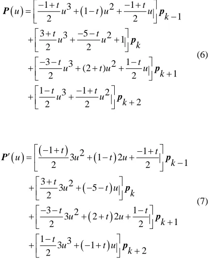
Unit vector T is obtained by solving normalized first derivative of loop curve as T(u)=P' (u)/| P'(u)|, according to the following process: first, expanding the Cardinal Spline equation (Eq.(4)) to get the expanded Eq.(6) and then solving its first derivative, shown as Eq.(7).

( )

(

)

1

1

2 2

3 3 5 2 ₁

2 2

3 3 _{(2 )} 2 1

1

2 2

1 ₃ 1 ₂

2 2 2 − + − +   =_ + − + _{ −}   + − −   +_ + + _   − − −   +_ + + + _{ +}   − − +   +_ + _{ +}   t t

u u t u u

k

t t

u u

k

t t

u t u u

k t t u u k P p p p p (6)

( ) (

)

(

)

(

)

(

)

(

)

1 ₂ 1

3 1 2

1

2 2

3 ₃ 2 ₅

2

3 ₂ 1

3 2 2

1 2 2 1 ₃ 3 1 2 2 − +  − +  =_ + − + _{ −}   +   +_ + − − _   − − −   +_ + + + _{ +}   −   +_ + − + _{ +}  

′ u t u t u t

k

t

u t u

k

t t

u t u

k

t

u t u

k P p p p p (7)

However, some specific points on the loop curve should be deleted where P'(u) is meaningless, such as when t equals to 1, P'(u)=(6u2-6u)pk+(-6u2+6u)pk+1 and the point is deleted where u equals to 0 or 1 because P'(u) is a zero vector in this case.

are located, and is a unit vector product of T (uq-1) and T (uq). The angle θ between T (uq-1) and T (uq)

always takes an acute angle, which ensures that the rotation angle of two adjacent sections does not exceed 90o. θ, R and Na can be obtained as the following equations,

( ) ( )

(

)

= _q ⋅ _q

θ T u T u (8)

( ) ( )

( ) ( )

− − × = × q q q q u u u u T T R T T (9)

a(uq)= ( θ)⋅ (uq−1)

N M R, N (10)

Where: M is the rotating matrix. Rotating matrix M can be obtained by Eq.(11).

(

)

(

)

(

)

(

)

(

)

(

)

(

)

(

)

11 12 13 21 22 23 31 32 33 2 11 12 13 21 2 22 23 31 32 ( ) 1 1 1 1 1 1 1 1 θ θ θ θ θ θ θ θ θ θ θ θ θ θ θ θ     =       = − + = − − = − + = − + = − + = − − = − − = − + x

x y z

x z y

x y z

y

y z x

x z y

y z

m m m

m m m

m m m

m R cos cos

m R R cos R sin

m R R cos R sin

m R R cos R sin

m R cos cos

m R R cos R sin

m R R cos R sin

m R R cos

M R,

(

)

m R cos cos

(11)

Where: Rx, Ry and Rz are component values of R on x,

y, z axis. Next, the bionormal unit vector B and normal unit vector N are solved by the following equations:

( )

( )

_{( )}

( )

_{( )}

a × = × q q q q q u u u u u T N B

T N (12)

( )

( ) ( )

_{( ) ( )}

T B (13)

With the proposed local frame above, unreasonable yarn rotation can be avoided to ensure superior 3-D

rotation matrix M(T,φ) where φ is in positive correlation with the distance between two continual points on the yarn path curve, namely φ=ω|P(uq -1)P(uq)|. ω is a parameter which has a positive

correlation with the twist effect.

Loop Surface Forming

When the yarn path curve and moving frame are solved, the section curve sweeps along the yarn path to form sets of section planes, shown as Figure 11. Section planes are defined by Eq. (14) and the spatial points on the section curves are obtained with Eq. (15) according to three dimensional coordinate transformation method [24]. The normal of the spatial points are same as that of section curve. For the circle section curve, the normal vector moves from center to circumference. The geometric effect of the yarn has a strong relationship to the geometry of the section curve For example, one circle results in a filament while numerous circles form a twisted yarn.

FIGURE 11. Loop surface forming model.

( )

(

( )

( )

)

C (14)

( )

( )

( ) ( )

( ) ( )

S P N B (15)

IMPLEMENTATION AND RESULTS

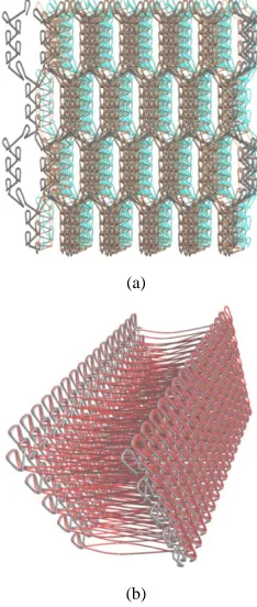
typed in first, and then the yarn path curve is drawn according to parameters associated with the Cardinal spline method. Afterwards, simulation parameters, including yarn thickness, yarn color, yarn geometry are set and section curves are formed to sweep along yarn path curve based on the moving frame and then rendered with OpenGL tools, forming the final 3-D warp-knitted fabric simulation effect. Simulation results for warp-knitted fabrics are used as examples to prove the method proposed above: 4 bars power-net (shown as Figure 12-a) and hex-net structures with fancy yarn (shown as Figure 12-b), two-bar tricot stitch fabric with twisted yarns (shown as

Figure 13), and double needle bed spacer fabric (shown as Figure 14). A double needle bed fabric is modeled as two opposed single needle bed fabrics.

(a)

(b)

FIGURE 12. Simulation of mesh structures. (a) power-net; (b) hex-net.

(a)

(b)

FIGURE 13. Simulation of structures with twisted yarns. (a) structure with more twist; (b) structure with less twist.

(a)

(b)

CONCLUSION

A method to simulate 3-D warp-knitted fabrics is proposed based on loop modeling with the Cardinal spline and recursive rotation moving frame. Spatial coverages of loops and inlays are simplified to three layers and one layer, respectively for visible lapping detection. Eight geometrical control points are defined for the stitched loop and three for the inlay. Using this method based on Cardinal spline, the centerline can be generated as long as the control points are given, facilitating the simulation of a variety of fabrics. Recursive rotation moving frame simulated a variety of fabrics and different yarn cross-sections well, avoiding abnormal twist. Further, the calculation process associated with this method is simple and easy to implement. Moreover, these methods can also be applied to the simulation of weaving and weft-knitted fabric. Twist deformation of loops caused by internal yarn forces and detailed brightness modeling (semi-dull, dull and bright) will be studied in future research.

ACKNOWLEDGEMENT

The authors acknowledge the financial support from the Innovation fund project of CIUI (Cooperation among Industries, Universities & Research Institutes) Jiangsu Province(BY2015019-31), Fundamental Research Funds for the Central Universities (JUSRP51625B) and A Project Funded by the Priority Academic Program Development of Jiangsu Higher Education Institutions(PAPD).

REFERENCES

[1] Başer G. Modeling of Complex Fabric Structures by Methods of Computer Simulation[J]. Journal of Textiles and Engineer, 2015, 2, 22(98).

[2] Dabiryan H， Jeddi A. Analysis of warp knitted fabric structure. Part I: A 3D straight line model for warp knitted fabrics. Journal of the Textile Institute, 2011, 102(12):1065-1074. [3] Postle R, Munden D L. Analysis of the

dry-relaxed knitted-loop configuration: part II: dimensional analysis [J]. Journal of the Textile Institute, 1967, 58(8): 352-365.

[4] Choi K F, Lo T Y. An energy model of plain knitted fabric[J]. Textile research journal, 2003, 73(8): 739-748.

[5] Kurbak A, Alpyildiz T. A geometrical model for the double lacoste knits[J]. Textile Research Journal, 2008, 78(3): 232-247.

[6] Kurbak A, Ekmen O. Basic studies for modeling complex weft knitted fabric structures Part I: A geometrical model for widthwise curling of plain knitted fabrics [J]. Textile Research Journal, 2008, 78(3): 198-208.

[7] Sherburn M. Geometric and mechanical modelling of textiles[D]. University of Nottingham, 2007.

[8] Yuksel C, Kaldor J M, James D L, Marcher S. Stitch meshes for modeling knitted clothing with yarn-level detail[J]. ACM Transactions on Graphics (TOG), 2012, 31(4): 37.

[9] Guo K, Wang X, Wu Z, et al. Modelling and Simulation of Weft Knitted Fabric Based on Ball B-Spline Curves and Hooke's Law[C]//2015 International Conference on Cyber worlds (CW). IEEE, 2015: 86-89. [10] Li Y L, Yang L H, Chen S Y, et al. 3D modeling

and simulation of fancy fabrics in weft knitting[J]. Journal of Donghua University (English Edition), 2012, 29: 351-358.

[11] Zhang L Z, Jiang G M, Miao X H, et al. Three-dimensional computer simulation of warp knitted spacer fabric[J]. Fibres & Textiles in Eastern Europe, 2012,20(3):56-60.

[12] Zhang L Z, Jiang G M, Gao W D. 3D simulation of two-bar warp-knitted structures[J]. Journal of Donghua University, 2009, 26(4): 423-428.

[13] Goktepe O, Harlock S C. Three-dimensional computer modeling of warp knitted structures[J]. Textile Research Journal, 2002, 72(3): 266-272.

[14] Durville D. Finite element simulation of textile materials at the fiber scale[J]. arXiv preprint arXiv:0912.1268, 2009.

[15] Wang G P. Comparison of three moving frames for SWEEP surface[J]. Journal of Computer Aided Design and Computer Graphics, 2001, 13(5): 455-460.

[16] Kyosev Y, Renkens W. Modelling and visualization of knitted fabrics[J]. Modelling and Predicting Textile Behaviour. Woodhead Publishing, 2009: 225-262.

[17] Liao T, Adanur S. 3D structural simulation of tubular braided fabrics for net-shape composites[J]. Textile Research Journal, 2000, 70(4): 297-303.

[19] Renkens W, Kyosev Y. 3D simulation of warp knitted structures–new chance for researchers and educators [C], 7th International Conference-TEXSCI, 2010.

[20] Goktepe O, Harlock S C. A 3D loop model for visual simulation of warp-knitted structures [J]. Journal of the Textile Institute, 2002, 93(1): 11-28.

[21] GM Jiang. Knitting Science[M]. China Textile & Apparel Press.2012:129.

[22] Zhang J, Baciu G, Cameron J, et al. Particle pair system: An interlaced mass spring system for real-time woven fabric simulation[J]. Textile Research Journal, 2012, 82(7): 655-666.

[23] Li X, Zhang A, Ma P, et al. Structural deformation behavior of Jacquardtronic lace based on the mass-spring model[J]. Textile Research Journal, 2016: 0040517516651103. [24] Donald Hearn, M. Pauline Baker, Warren R.

Carithers. Computer Graphics with OpenGL, Fourth Edition. Publishing House of Electronics Industry.2014, 11:230 -321.

AUTHORS’ ADDRESSES Aijun Zhang

Xinxin Li Sha Sha Gaoming Jiang

Engineering Research Center for Knitting Technology