Target Recognition in SAR Image via Keypoint based Local Descriptor—Foundation

(1)

Target Recognition in SAR Image via Keypoint

based Local Descriptor—Foundation

Ganggang Dong and Jocelyn Chanussot, Fellow, IEEE

Abstract—This paper considers target characterization and recognition in radar images with keypoint-based local descriptor. Most of the preceding works rely on the global features or raw intensity values, and hence produce the limited recognition performance. Moreover, the global features are sensitive to the real-world sources of variability, such as aspect view, configu-ration, and incidence angle changes, clutter, articulation, and occlusion. Keypoint-based local descriptor was developed as a powerful strategy to address invariance to contrast change and geometric distortion. This property inspires us to investigate whether the family of local features are relevant for radar target recognition. Most of the preceding works typically devote to finding the correspondences between a collected image and a reference one. The representative applications include image register and change detection. Little work was pursued to target recognition in SAR images. This is because the huge number of local descriptors resulting from radar images make the computational cost and memory consumption unacceptable. To handle the problems, this paper develops two families of methods. The proposed methods are used to achieve target recognition by means of local descriptors. Our first solver refers to building multiple linear regression models, and addresses the problem by the theory of sparse representation. The second scheme rebuilds a new feature by the feature quantization skill, from which the inference can be drawn. Multiple comparative studies are pursued to verify the performance of detectors and descriptors popularly used. The source code was publicly released on https://ganggangdong.github.io/homepage/.

Keywords—Target recognition, SAR, keypoint, local descriptor, sparse representation, feature quantization, classification.

I. INTRODUCTION

W

ITH the development of integrated circuit and manufac-turing technology, the resolution of synthetic aperture radar in range and azimuth is capable to achieve target recog-nition. However, images taken from various sensor platforms are too huge to be handled by analyst timely. This situation produces an urgent need for automatic image interpretation [1], [2]. Though many works have been initiated to provide a base-line knowledge of target scattering characteristics, automatic target recognition in radar image is still far from being solved due to the complicated imaging condition. It is nevertheless

This works was supported by the National Natural Science Foundation of China under Grant 61601481, and by the Hunan Provincial Science Foundation of China under Grant 2016JJ3023.

Dr. Ganggang Dong is with National Laboratory of Radar Signal Processing, Xidian University, Xi’an, China, and with School of Electronic and Informa-tion Engineering, Xi’an, China (e-mail: [email protected]).

Prof. Jocelyn Chanussot is with with the engineering school on Energy, Water and Environment (ENSE3) of the Grenoble Institute of Technology, Grenoble, France (e-mail: [email protected]).

worth to be addressed because this technology gives great potential for the civil use as well as the military application.

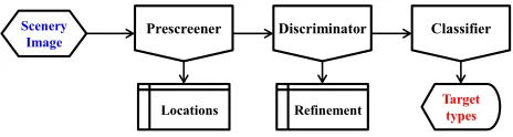
The typical system for radar target recognition is usually composed of three separate phases, prescreening, discrimina-tion, and classification [3]. The work mechanism is shown in Fig. 1, where the input is a scenery of radar image, and the output are the target types. The prescreening stage produces the candidate targets by examining the amplitude of radar signal pixel by pixel [4]. The discrimination stage locates the candidate accurately and generates the orientations [5]. The natural clutter false alarms are rejected by texture features. The classification stage predicts the identifications.

Activation Decode

Target types

Scenery Image

Locations Refinement

Prescreener Discriminator Classifier

Fig. 1. The mechanism of automatic target recognition from radar image.

A. Background

This paper considers the classification subsystem. The input is a chip image cropped from the scenery, while the output is the identification. The chip image inputted usually contains a single target, radar shadow, and background, as visually shown in Fig. 2. In the conventional methods, the prediction of target type is achieved by feeding a designed feature into a trained classifier. The recognition performance is therefore dependent on the representation and classification scheme.

10 20 30 40 50 60 70 80 90 10

20 30 40 50 60 70 80 90

10 20 30 40 50 60 70 80 90 10

20 30 40 50 60 70 80 90

10 20 30 40 50 60 70 80 90 10

20 30 40 50 60 70 80 90

Fig. 2. Illustration of target and radar shadow for radar chip image.

1) Feature Representation: The signature information that distinguishes one target from another is fundamentally deter-mined by the interactions between the incident radar waveform and target physical structure. For radar imagery, the backscat-tered signal results from multiple scattering mechanisms, e.g., direct backscatter, single-direction double bounce, return-direct multi-bounce, and high-order multiple bounce. The unique imaging mechanism makes feature extraction from radar image

(2)

much more difficult. The present approaches can be reviewed as follows.

Intensity values. The early methods achieve target recog-nition by the raw intensity values or the enhanced image. The distance between two sets of pixel values (or enhanced values) are used to make the decision. L. Novak et al. pro-pose a new super-resolution image-processing technique that enhances SAR image resolution [6]. The enhanced image is fed into a MSE-classifier to predict the target type. Q. Zhao and J. Principle design a support vector machine, into which the raw intensity values are pushed directly [7]. J. Thiagarajan propose to feed the randomly projected coefficients of image into sparse representation-based classifier [8]. This kind of methods are dependent on the trained classifier more and on feature less.

Projection coefficients. This kind of methods refer to con-structing a linear subspace by the intensity vectors. A feature representation is then defined by the projected coefficients, such as principal component analysis, independent component analysis. The physical meaning is therefore ambiguous. M. Liu et al. present a statistical model embedding the locality preserving property to extract the maximum amount of desired information from the data [9]. Y. Huang et al. propose to preserve the global and local discriminative information based on the tensor representation [10]. Z. Cui et al. generate the pattern feature of SAR image by a variant of non-negative matrix factorization [11].

Filter banks.In some works, the feature is defined by a set of filter banks, such as Fourier transform, Gabor filters, and the analytic signal. R. Patnaik and D. Casasent achieve target recognition by the correlation patter recognition strategy [12], [13]. A set of correlation filters are first generated by Fourier transformed coefficients of the training. The decision is made according to the correlation response between the query and the generated filters. G. Donget al.develop a new method for target recognition [14]–[16]. The target signature information is characterized by an extended analytic signal, the monogenic signal [17], [18]. Sparse representation modeling is built to implement target classification.

Geometric features.The geometric feature means the shape, edge, size of target or radar shadow. This family of features are mainly dependent on the fine segmentation of radar image, which is still an open problem now. J. Parket al.discriminate target from clutter by some designed geometric features, such as the minimum projected length, the contrast of the projected length, the energy of the projected length in the frequency domain [19]. J. Zhuet al.introduce a famous trick of computer vision, shape context, to exploit the distinguishing characters of the ship targets from radar image [20]. They jointly consider the topology and intensity of scattering points of ship.

Statistical feature. Some researchers employ the image statistics for target recognition, such as the various statistical moment. J. Singh and M. Datcu utilize a chirplet-derived transform and fractional Fourier transform to generate a com-pact feature descriptor for single-look SAR images [21]. The statistical response resulting from the projections on different planes of the joint time-frequency space is easy to be ana-lyzed. M. Anoon and G. Rezai-rad generate a representation by the Zernike moments [22]. The resulting feature is of

linear transformation invariance and robustness in the presence of the noise. The similar thought was employed in [23]. P. Bolourchi et al. propose a feature descriptor by Radial Chebyshev moment, a discrete orthogonal moment with some distinctive advantages [24].

Learned feature. Target recognition via the learned fea-ture is a recent research hotspot. S. Chen et al. propose to learn the hierarchical features from massive training data by convolutional neural networks [25]. The similar thoughts can be found in [26]–[28]. S. Deng et al. introduce stacked autoencoder for target classification [29]. The reshaped image is specified as the visible layer, while the latent states are used to classification. Though performed well, this family of features are computationally unattractive. In addition, they present a heavy demand for the hardware configuration.

Scattering center model. Radar energy backscattered from the object contains the key information that distinguishes one target from another. An intuitive idea is to define a feature by the scattering center models. L. Potter and R. Moses pursue the preliminary studies [1]. They present a framework for feature extraction predicated on parametric models for the radar returns. The developed models are motivated by the scattering behavior predicted by the geometrical theory of diffraction. J. Zhou et al. propose a global scattering center model established offline using range profiles at multiple viewing angles, with which features at different target poses can be conveniently predicted. B. Ding et al.introduce a new statistics-based metric to measure the distance between the attributed scattering center models [30]. This family of features are difficult to be flexibly generalized.

Though multiple schemes were presented previously, feature extraction is still far more to be solved, especially for the real-word applications. The invariance to the real-world sources of variability should be further studied.

2) Classification Learning: The extracted feature is used to determine the class to which a detected target belongs by the knowledge learned from the training. It is a typical application of patter recognition in radar image. The current approaches are reviewed as follows.KNNis of the most fundamental and explicit strategy. It predicts the class membership according to the similarity between the probe and the gallery. The key is how to define an appropriate distance metric for the de-signed feature.Kernel-based Classifier. This family of method projects the original data into an implicit feature space whose dimension can be as high as possibly or even infinite. The class separability can be then enhanced. The most representative is support vector machine learning [7].Regression analysisskills are popularly used in neural network configuration [25], [29]. It models the relationship between a scalar dependent variable and a set of explanatory variables. The response is the target type, whose output is the probability of the class label taking one each of the possible values. Sparse representation-based classification is a specialty of regression analysis [32].

B. Contributions

(3)

the real-world source of variability. To handle the problems, this paper considers keypoint-based local descriptor for target recognition. Two families of methods, following the thought of sparse representation and feature quantization, are developed. The pipeline is displayed in Fig. 3. To our knowledge, the relevance of keypoint-based scheme in target recognition has been investigated seldom. We aim at studying to which extent the local descriptor can improve the recognition performance. We intend to open a new door for target recognition under the non-literal conditions. Our contributions therefore include:

• the comprehensive review of the preceding works on feature extraction from radar image,

• the tune of keypoint-based local descriptor for radar target recognition,

• the development of two families of schemes to imple-ment target classification with the local descriptor, • the evaluation of proposed strategy with multiple

com-parative studies.

0 20 40 60 80 100

10 20 30 40 50 60 70 80 90

-2.5 -2 -1.5 -1 -0.5 0 0.5 1 1.5 2 2.5 -2 -1.5 -1 -0.5 0 0.5 1 1.5 2

0 20 40 60 80 100

10 20 30 40 50 60 70 80 90

-2.5 -2 -1.5 -1 -0.5 0 0.5 1 1.5 2 2.5 -2 -1.5 -1 -0.5 0 0.5 1 1.5 2

-2.5 -2 -1.5 -1 -0.5 0 0.5 1 1.5 2 2.5 -2 -1.5 -1 -0.5 0 0.5 1 1.5 2 Dictionary Sparse Representation Feature Quantization Scheme 1 Scheme 2 Decision

Training Query

Basis Vectors

Visual Words

0 20 40 60 80 100

10 20 30 40 50 60 70 80 90

0 20 40 60 80 100

10 20 30 40 50 60 70 80 90

0 20 40 60 80 100

10 20 30 40 50 60 70 80 90

Fig. 3. Pipeline of proposed framework.

C. Organization

The rest of this paper is organized as follows. Section II reviews the representative keypoint detectors and local descrip-tors. Section III develops two families of methods for target recognition. Section IV verifies the proposed schemes with multiple comparative experiments. Section V concludes this paper.

II. KEYPOINT-BASEDLOCALDESCRIPTOR

Most of the previous studies achieve target recognition by the global feature. They are not effective to the non-literal conditions. The recent development on machine learning prove that the local region description could produce very powerful cues. Compared to the global feature, the keypoint-based local descriptor is much more robust to real-world source of variability. This property motivates us to achieve target recognition with the local descriptor. This section provides a simple review of related studies from two aspects, the detection of keypoint and the representation of local feature.

A. The Detection of Keypoint

Keypoint detection refers to checking image pattern which differs from the immediate neighborhood. The fashion of rep-resentation could yield a high repeatability, i.e., the keypoints can be extracted reliably and are often found again at the similar locations in other images of the same object or scene.

For radar chip image, the keypoints are undoubtedly located in the target imaging region, or radar shadow. The popularly used approach to keypoint detection includes difference of Gaussian (DoG), Harris corner detector, Hessian blob-like structure detector, and the variants.

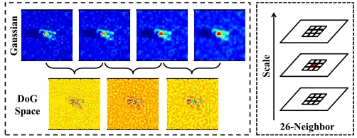
1) Difference of Gaussian: DoG is an approximation of Laplace of Gaussian [33], and much faster to compute. A scale-space S(x, y, σ)is first built by convolving the imageI(x, y)

with a Gaussian low-pass filter G(x, y, σ)parameterized by a standard deviation σ,

S(x, y, σs) =G(x, y, σs)∗I(x, y).

whereσsis a function of indexs={0,1, . . . , smax-1}. DoG

images is the difference between two successive layers D(x, y, σs) =S(x, y, σs+1)− S(x, y, σs).

To achieve scale-invariance, image pyramids are usually built. The number of octave is determined by the size of image. Image in the higher-order octave is obtained by downsampling the one of the previous octave in a factor of 2. Keypoint is defined as the local extrema in 3-dimension space (x, y, σ). It is checked by comparing every pixel to the eight neighboring pixels in the current scale and the nine pixels in the scales above and below. If a pixel is larger or smaller than all of its neighbors, it is accepted as a preliminary keypoint candidate. The implementation flow of DoG is pictorially shown in Fig. 4.

0 20 40 60 80 100 10 20 30 40 50 60 70 80 90

0 20 40 60 80 100 10 20 30 40 50 60 70 80 90 DoG Space G au ss ia n S ca le 26-Neighbor

Fig. 4. The illustration of DoG detector. The pixel (in red) is compared to the eight neighbors in current scale, and the nine neighbors in the previous and next scales.

2) Harris Detector: Harris corner detector is probably one of the earliest method for keypoint detection [34]. It is based on the eigenvalues of second-moment matrix (or autocorrela-tion). The candidates with low contrast are then filtered by thresholding the values of the built matrix,

M(x, y, σ) = det(Ha(x, y, σ))−λ·trace(Ha(x, y, σ))2.

The Harris matrix is

Ha(x, y, σ) =

S2

x(x, y, σ) {Sx· Sy}(x, y, σ)

{Sy· Sx}(x, y, σ) Sy2(x, y, σ)

where Sx, Sx are the convolution of the Gaussian first-order

derivative _∂x∂ G, ∂

∂yGwith imageI(x, y). The parameterλis to

balance the determinant and trace of Harris matrix, and usually set between 0.04∼0.06.

(4)

scale. Mikolajczyk and Schmid further present a refined strat-egy, Harris-Laplace detector, by which scale-invariant feature detectors with high repeatability can be created [36]. The location of keypoint is selected by the determinant, while the scale is determined by the Laplacian operator.

3) Hessian Detector: Hessian detector defines the keypoints as the ones localized in space at the local maxima of the Hessian determinant and in scale at the local maxima of the Laplacian-of-Gaussian. For 2-D functionI(x),x= [x, y], the second-order Taylor’s expansion is expressed as

I(x0+4x)≈I(x0) +4xT∇I(x0) +4xTH(x0)4x

The Hessian matrix at each point location is

He(x, y, σ) =

Sxx(x, y, σ) Sxy(x, y, σ)

Syx(x, y, σ) Syy(x, y, σ)

whereSxx,Sxy,Syy are the convolution of Gaussian

second-order derivative _∂x∂22G,

∂2

∂x∂yG, ∂2

∂y2G with image I(x, y). The

blob-like structures are detected by the determinant of Hessian matrix and the trace of Hessian matrix (Laplacian),

det(He) =SxxSyy−λ0· SxySyx

whereλ0 is a weight parameter. For the 9×9 filter in size and σ= 1.2, the weight parameter is approximated as

kSxy(1.2)kFkDxx(9)kF

kSxy(1.2)kFkDxy(9)kF

= 0.912_w0.9

where Dxx, Dxy, Dyy are the approximations of Sxx, Sxy,

Syy1. By assigning each detected keypoints its own

character-istic scale, the scale invariance can be achieved.

To boost the computational efficiency, H. Bay et al. also present a fast version of Hessian-Laplace detector, Fast-Hessian [37], [38], where the integral image is used to cir-cumvent image derivative operations.

4) Features from Accelerated Segment Test: E. Rosten and T. Drummond propose a novel efficient approach to corner detection, features from accelerated segment test (FAST) [39], [40]. The designed segment test criterion operates by consid-ering a circle of sixteen pixels around the keypoint candidate, as illustrated in Fig. 5.

6 12

5 13

4 14

15 3

1 2 16

9 8 10

11 7

Fig. 5. Illustration of FAST. The pixel in red is the center of a candidate corner, while the 16 pixels in circle are considered in corner detection.

1_{The detail derivation can be found in the preceding works [37].}

A corner pis defined if there exists a set of n contiguous pixels in the circle which are all brighter than the intensity of the candidate pixel Ip plus a threshold τ, or all darker than

Ip −τ. The parameter of n is set as twelve, with which a

very large number of candidates can be excluded. Considering the computational efficiency, only four neighborhood pixels at {1,5,9,13}-site are tested. Therefore, if a keypoint is detected, then at least three of these values should all be brighter than Ip+τ or smaller thanIp−τ. For a candidatep, these sixteen

sites on the circle are noted ass1, s2, . . . , s16∈ Np. The pixels

at those sites can be categorized as one of three states,

Isi ⇒

( _darker _I

p6Ip−τ

similar Ip−τ < Ip< Ip+τ

brighter Ip>Ip−τ

The detected keypoints are then refined by non-maximal sup-pression trick.

B. Feature Representation around Keypoint Detected

Have detected keypoint, a pair of pixel coordinates, another key issue is how to characterize the neighborhood around the point, i.e., define an invariant feature descriptor.

1) SIFT: SIFT may be the most popularly used descrip-tor [41]. It is defined as the histogram of gradient orientation weighted by magnitude and a Gaussian window. The dominant orientation is estimated to achieve rotational invariance.

For image pyramid S(x, y, σ), the gradient magnitude and orientation are computed at all scales and octaves,

Magnitude⇒qS2

x+Sy2

Orientation⇒arctan Sy

Sx

whereSx= ∂_∂xS andSy= ∂_∂yS are the partial derivatives along

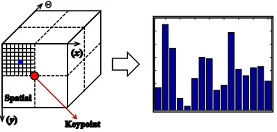
x- andy-axis directions. The gradient orientation weighted by magnitude and a Gaussian window is used to produce a 3-D histogram. The first two dimensions correspond to the spatial location, and the additional dimension to gradient orientation. Each pixel within the local region contributes to the histogram depending on the location, gradient orientation and magnitude. Image gradient computed around every keypoint is integrated to the 3D histogram, resulting 2×2×2 bins, each of which is incremented by gradient magnitude multiplied by a weight inversely related to distance between the location and keypoint. The peak value of histogram and those ones larger than 80% peak are defined as the dominant orientation. A square neighborhood around each point with a size depending on the scale is cropped. It is inversely rotated by the dominant orientation. To assure the scale invariance, image gradients are calculated at the same scale to which the keypoint belongs. Local descriptor is obtained by concatenating the histograms, producing a 128-element-vector, as shown in Fig. 6.

(5)

Θ

Spatial

Keypoint

2 4 6 8 10 12 14 16 0 10 20 30 40 50 60 70

(x)

(y)

Fig. 6. The generation of SIFT descriptor.

are set according to the task at hand. The central circle region is handled as a single bin, while the outer circular regions are divided into 8 bins equally distributed along angular direction, in each of which the gradient orientation weighted by magnitude is quantized into 8 levels. The generation of histogram is similar to SIFT. The local descriptor is obtained by concatenating the histograms of all sectors. GLOH refines the division of location, and hence results in an improvement on performance, as proved in [42]. The comparison of SIFT and GLOH are pictorially shown in Fig. 7.

-2.5 -2 -1.5 -1 -0.5 0 0.5 1 1.5 2 2.5 -2 -1.5 -1 -0.5 0 0.5 1 1.5 2

-2.5 -2 -1.5 -1 -0.5 0 0.5 1 1.5 2 2.5

-2 -1.5 -1 -0.5 0 0.5 1 1.5 2

-2.5 -2 -1.5 -1 -0.5 0 0.5 1 1.5 2 2.5 -2 -1.5 -1 -0.5 0 0.5 1 1.5 2

SIFT GLOH

Orientation

Fig. 7. Square grid for SIFT and log-polar sector for GLOH.

3) Adaptive Binning Strategy: The conventional descriptor usually divides the neighborhood around keypoint into some fixed cells, e.g., 4×4 grids for SIFT, 1+8+8+8 sectors for GLOH, in each of which the gradient orientation is quantized. The levels of quantization for gradient orientation is also fixed. This mode of quantization may reduce the discriminative power. A. Sedaghat and H. Ebadi propose to separate the inner circle and the outer circular regions into different radial sectors. The gradient orientations within each sector is quantized into different levels [43].

For each keypoint detected, its neighborhood is divide inton non-overlapping circular rings,R1,R2, . . . ,Rn, as similar to

GLOH. Each circular region Ri is then divided intoNi cells

equally distributed along the angular direction {Ri(j)}Nj=1i .

The gradient orientations in Ri(j) are further quantized into

kilevels of histogram,i.e., the level of quantization is different

from cell to cell, as shown in Fig. 8. The descriptor is obtained by combining the histograms. The dimension of feature descriptor isP

iNiki.

4) DAISY: Engin Tola et al. develop a new local descrip-tor, DAISY [44], [45]. It circumvents the weighted sums of gradient norms by convolutions of the gradients in specific directions with Gaussian filters.

① R11 R12 R13 R14 R15 R21 R22 R23 R24 R25 R26 R27 R28 R31 R32 R33 R34 R35 R36 R37 R38 R39 R310 ③ ④ ⑤ ⑧ ⑦ ① ② ② ③ ④ ⑤ ⑥ ⑥ ⑦ ⑧

GLOH ABSIFT

Fig. 8. Illustration of GLOH and AB-SIFT. GLOH only divides the outer circular regions along angular directions, while AB-SIFT separates both the inner circle and the outer circulars into several sectors.

For chip image I(x, y), a set of orientation maps can be defined,Oi(x, y) =

∂I ∂i

+

, whereiis the quantized direction,

and (·)+ = max{·,0}. The orientation maps are convolved

with Gaussian kernel parameterized byσto generate different size of local regions,

Oiσ(x, y) =Oi(x, y)∗ Gσ(x, y).

DAISY is defined as a vector whose entries are the coefficients resulting from the convolved orientation maps located on concentric circles centered on the location,

hσ(x, y) = [O1σ(x, y),O

σ

2(x, y), . . . ,O

σ N(x, y)].

Considering M circular cells, the descriptor is obtained by concatenating the normalized vectors

[hT

σ1(x, y), h

T

σ1(d1(x, y, R1)), . . . , h

T

σ1(dn(x, y, R1))

hT

σ2(d1(x, y, R2)), . . . , h

T

σ2(dn(x, y, R2))

.. . hT

σM(d1(x, y, RM)), . . . , h

T

σM(dn(x, y, RM))]

where dj(x, y, Ri) denotes the sites with Ri distance from

(x, y)along thej-direction. The orientations are quantized into n levels.

5) SURF: H. Bay et al. present an improved version of Hessian detector, Fast-Hessian, by which a local descriptor, Speeded-Up Robust Features is defined [37], [38]. They first detect blob-like structure with the Hessian matrix, i.e., a second-order derivative of Gaussian filtered image. The deriva-tive operation is achieved by means of integral image. The local descriptor is defined as the distribution of first-order Haar wavelet response.

(6)

Denote byhx,hythe Haar wavelet response in horizontal and

vertical directions. The local descriptor is formed as

X

hx,

X

hy,

X

|hx|,

X

|hy|

T

.

III. CLASSIFICATION

Keypoint-based local descriptor is initially developed to find the correspondences between a pair of images. The representative application includes image register and change detection. Though studied widely, little work is devoted to radar target recognition. The local descriptors resulting from radar images may be the order of millions, and hence could not be handled as usual. To solve the problem, this paper proposes two methods. The first casts the recognition problem as one of classifying among multiple linear regression models [32]. The latter produces a single new feature for each image by encoding the local descriptors.

Given N labeled images I1, I2, . . . , IN from K distinct

classes, the task of target recognition is to predict the class membership of query using the knowledge learned from the labeled ones. For image Ii, we extract the local descriptors

V1

i, V

2

i, . . . , V ni

i around ni keypoints. The total number of

local descriptors available for training is n = P

ini. Target

recognition refers to predict the class identity ofIq according

to its local descriptors V1

q,Vq2, . . . ,V nq

q .

A. Solver 1: Sparse Representation

Our first solver proposes to build multiple linear regression models with the local descriptors. The descriptors available for training play the role of regressor, while the one of query is the response. The regression coefficients is obtained by optimizing `1-norm minimization. The theory of sparse representation

offers the key to address the problem [32]. We first represent the descriptors extracted from queryVi

q as a linear combination

of those resulting from the training, Vi

q=V11α11+V12α21+· · ·+V

n1

1 α

n1

1 +

V1 2α

1 2+V

2 2α

2

2+· · ·+V

n2

2 α

n2

2 +· · ·

V1

Nα

1

N +V

2

Nα

2

N+· · ·+V nN

N α nN

1

(1)

where [α1

1, α21, . . ., α12, α22, . . ., α1N, α2N, . . . , α nN

N ] are the

regression coefficients. This problem is incapable to be handled directly due to the huge number of descriptors, making the computation and memory unacceptable. A feasible method is to represent the query only by the related descriptors, and ignore the remaining. Following this thought, this paper develops a prescreener, with which the descriptors unrelated are filtered out. The preserved samples are used to represent the query. The key issue is therefore to design the prescreener.

For each descriptor of query Vi

q, this paper first computes

the linear correlation response with all of the local descriptors available for training,

ri= (Vqi) T_[_V1

1,V 2 1, . . . ,V

n1

1 , . . . ,V 1

N,V

2

N, . . . ,V nN

N ].

The (dis)similarity between a pair of local descriptors is mea-sured by the Euclidean distance metric. The other measurement could play a similar role. To filter the redundancy out, only the

most correlated descriptors are kept, while the remaining are ignored. We sort the correlation response ri in a descending

order, and hold the former descriptors P = b1, b2, . . . ,

bL. They are employed as the basis vectors to represent the

descriptor of query Vi

q =b1α1+b2α2+· · ·+bLαL=Pα (2)

whereα1,α2, . . . ,αLare the weights. The number of atoms in

P is much smaller than the ones available for training,Ln. The computational cost is then greatly alleviated. Notedly, the dictionaryP is different from descriptor to descriptor.

According to the theory of sparse representation, we expect that most of the entries forαare zero except those associated with the real class identity of query. This is realized by op-timizing`0-norm minimization problem. Thanks to the recent

development of compressed sensing [46], the solution of `0

-norm minimization is equal to the one of`1-norm minimization

if αis parsimonious enough,

min

α kαk1 s.t. kV i q− Pαk

2

2< ε (3)

wherek·k1sums the absolute value of entries. It can be further

converted to the unconstrained optimization problem,

min

α

kαk1+λkVqi− Pαk22 (4)

where the parameter λ balances the fidelity and the sparsity. The optimal representation αˆ is used to calculate the recon-struction error

ej_i =Vi

q−δj(P) ˆαj, j= 1,2, . . . , K (5)

where the functionδj(P)is designed to select those atoms

as-sociated with thej-th class, andαˆjis the corresponding weight

coefficients. The overall residual is obtained by accumulating (5) over the descriptors,e= Pnq

i e

1

i,

Pnq

i e

2

i, . . . ,

Pnq

i e K i

. The class membership of query Iq is estimated by finding the

minimum overall reconstruction error arg minj

n P

ie j i

o

. Since only a small portion of descriptors related are em-ployed to build the multiple linear regression models, the proposed method has the advantage of simplicity and com-putational efficiency.

B. Solver 2: Feature Quantization

Different from the first method, we propose another solver by feature quantization. It treats an image as a collection of unordered descriptors extracted from the local region, and quantizes them over the “visual words” [47]. A new compact histogram is produced by a predefined codebook for semantic classification.

1) Bag of Visual Words (Bow): BoW represents the local descriptors by a set of visual words. A codebook composing of visual words is first generated by a batch of descriptors. They can be the overall descriptors available, or randomly selected from the training set. Denote byV(1),V(2), . . . ,V(n0₎ the batch of feature selected from the training set. K-means clustering algorithm is employed to generate a codebook

minCP

n0

(7)

are the clustering centers. The prototype of BoW commits each descriptor to the nearest atom. The hard assignment is too restrictive, and hence produces a coarse reconstruction. Yang et al. [48] propose to relax the constraint by sparse coding (SC), enforcing the representation to be with a small number of nonzero entries,

min

C,α n0

X

j=1

kV(j)− Cαk22+λkαk1 (6)

Wang et al. [49] present another trick, locality-constrained linear coding (LLC) by projecting the descriptor into its local-coordinate system with a locality constraint,

min

C,α n0

X

j=1

kV(j)− Cαk22+λkdj⊗αk22 (7)

where⊗denotes the element-wise multiplication, and

dj= exp

[d(V₍_j₎,C₁), d(V₍_j₎,C₂), . . . , d(V₍_j₎,C_m)]T

σ

is a constraint composing of the distance to atoms.

2) Fisher Vectors (FV): Since building an universal and compact vocabulary seems irreconcilable, an alternative idea is to depart the generation of codebook. F. Perronnin et al. pro-pose to apply Fisher kernels for image categorization [50], [51]. The core is to characterize a signal with a gradient vector derived from a probability density function which models the generation process of the signal. Gaussian Mixture Models which approximates the distribution of image features is usually employed.

Denote by V = [V1,V2, . . . ,VJ] a set of local descriptors

available, and Θ = {ωi, µi,Σi}Ni=1 the GMM parameters to

be estimated, corresponding to weight, mean, and covariance matrix. Each Gaussian distribution represents a word of visual vocabulary. Under an independence precondition, it is capable to produce

F(V|Θ) =

J

X

j=1

logp(Vj|Θ) =

J

X

j=1

log(

N

X

i=1

ωipi(Vj|Θ)) (8)

where the componentpi(·)is thei-th Gaussian distribution

pi(x|Θ) =

1 p

(2π)D_|_Σ

i|

exp(−0.5(x−µi)TΣ−i1(x−µi)).

Assuming the diagonal covariance matrices, σ_i2 =diag(Σi),

only the derivatives ∂F_∂ω(V|Θ)

i ,

∂F(V|Θ)

∂µi ,

∂F(V|Θ)

∂σi are

consid-ered. This leads to the representation which captures the aver-age first and second order differences between local features and each of the GMM centers,

Φ(1)_k = 1

N√ωk N

X

p=1

αp(k)

V_p−µ_k

σk

Φ(2)_k = 1

N√2ωk N

X

p=1

αp(k)

(V_p−µ_k)2

σ2

k

−1

whereαp(k)is the soft assignment weight of thep-th feature

to the k-th Gaussian distribution. The new feature is obtained by stacking the difference Φ(1)₁ ,Φ(2)₁ , . . . ,Φ(1)_N ,Φ(2)_N .

IV. EXPERIMENTS ANDDISCUSSIONS

This paper develops two kinds of methods to implement target classification by local descriptor. The proposed strategy is validated on MSTAR SAR images, a database collected by a 10 GHz SAR sensor with 1 ×1-foot resolution in range and azimuth. Images of four military vehicles, BMP2, T72, BTR70, and T62 are employed, among which BMP2 and BTR60 are armored personnel carriers, while T72 and T62 are main-battle tanks. BMP2 and T72 have several variants with the structural modifications, noted by the series number, SN 9563, SN 9566, SN c21 for BMP2, SN 132, SN 812, SN s7 for T72. BTR60 and T62 are of single configuration. The standard, SN 9563 and SN 132 taken at a 17◦depression angle are used for training, while the remaining collected at a 15◦ depression angle comprise the testing set. Significant changes of configuration and depression angle are present, as detailed in TABLE I. The original images are of around 128×128 pixels in size, and standardized as 96×96 pixels by cropping the center patches. All experiments are performed on Matlab 2015a.

TABLE I. THE NUMBER OF ASPECT VIEW IMAGES FORBMP2, BTR70, T62,ANDT72.

Depr. BMP2 T72 BTR60 T62 Total

17◦(Gallery) 233 (SN 9563) 232 (SN 132) 256 299 1020 15◦(Probe) 196 (SN 9566)

196 (SN c21)

195 (SN 812)

191 (SN s7) 195 273 1246

A. The Detection of Keypoint

We first evaluate the performance of representative detectors. We aim to studying whether these methods could seek keypoint from radar image, and whether the local descriptors around the keypoints could exploit target signature information.

We provide a set of instance on keypoint detection. Fig. 9 draws the detection maps obtained using DoG, Hessian, Harris-Laplace, and Hessian-Laplace2_{. We found that the keypoints}

detected are mainly located in target imaging region, cor-responding to the local scattering centers. The number of keypoints produced by DoG is much more than the other detectors. Keypoints generated by Hessian-Laplace detector are more than Hessian. Those points located in main gun of tank have also been detected.

Fig. 10 shows the detection chart of FAST on the same image3_{. The threshold value}_τ _{is set as 0.25, 0.2, 0.15, and 0.1.}

With the threshold value decreased, the number of keypoints detected are increased. The smaller the threshold, the more the number of keypoints detected. Most of these keypoints are located in target imaging region, similar to the previous maps. The small threshold value usually produces some keypoints in the site of speckle.

2_VLFeat_{toolkit is used to implement the detectors.}

3_{The function ‘fast9’ is employed. More information can be found in the}

(8)

0 20 40 60 80 100 10

20 30 40 50 60 70 80 90

0 20 40 60 80 100 10

20 30 40 50 60 70 80 90

0 20 40 60 80 100 10

20 30 40 50 60 70 80 90

0 20 40 60 80 100 10

20 30 40 50 60 70 80 90

Fig. 9. The detection maps obtained by DoG, Hessian, Harris-Laplace, and Hessian-Laplace. The keypoints are marked by pentagram in red.

0 20 40 60 80 100 10

20 30 40 50 60 70 80 90

0 20 40 60 80 100 10

20 30 40 50 60 70 80 90

0 20 40 60 80 100 10

20 30 40 50 60 70 80 90

0 20 40 60 80 100 10

20 30 40 50 60 70 80 90

Fig. 10. Keypoints detected by FAST with four different threshold values. The keypoints detected are noted by asterisk in yellow.

The average number of keypoints detected from the whole training set is then given. To study whether the number of keypoint is related to target pose, the aspect view is divided into four ranges, as detailed in TABLE II. We found that Harris-Laplace detector produces the least number of keypoints consistently, while FAST detector always seeks the most number of points. For BMP2, the number of detected points produced from Angle3is much more than the remaining angle

range. For BTR60, T72, and T62, the number of detected points is irregular. Hence, we could come the conclusion that the number of keypoints detected is not related to target pose.

TABLE II. THE NUMBER OF KEYPOINTS DETECTED FROM FOUR

CLASSES OF RADAR IMAGES. ANGLE1, ANGLE2, ANGLE3, ANGLE4

REFERS TO IMAGES WITH POSE FALLEN IN THE RANGE OF0◦∼90◦,

91◦_∼₁₈₀◦_,₁₈₁◦_∼₂₇₀◦_,₂₇₁◦_∼₃₆₀◦_.

Detector DoG Hessian HarrisL HessianL FAST1 _FAST2

BMP2

Angle1 14.84 12.98 6.07 19.72 31.77 42.59

Angle2 14.73 14.65 6.87 22.18 36.07 48.02

Angle3 18.06 17.69 8.51 26.33 40.06 52.57

Angle4 17.23 12.49 6.41 18.31 28.95 39.05

Overall 16.14 14.31 6.90 21.43 33.95 45.24

BTR60

Angle1 15.34 19.87 8.79 30.52 40.47 55.24

Angle2 14.88 17.96 8.46 27.39 41.57 55.13

Angle3 14.92 18.73 8.53 31.67 48.41 63.53

Angle4 18.05 18.95 8.75 29.19 44.68 59.81

Overall 15.87 18.91 8.64 29.66 43.63 58.28

T72

Angle1 15.40 16.63 7.50 21.63 37.18 48.21

Angle2 17.16 16.72 8.09 23.13 39.74 51.40

Angle3 16.65 16.28 7.15 22.43 39.25 51.93

Angle4 13.65 13.22 6.57 18.25 31.80 42.77

Overall 15.75 15.77 7.36 21.43 37.08 48.65

T62

Angle1 12.45 21.55 11.38 37.45 56.07 72.19

Angle2 12.43 19.12 10.43 38.08 55.30 71.14

Angle3 13.09 22.38 11.16 41.78 62.65 79.33

Angle4 13.50 24.10 12.06 38.43 58.79 75.71

Overall 12.87 21.78 11.25 39.00 58.29 74.69

We further quantitatively assess the detectors on recognition performance. The local descriptors extracted from the training

images are used to predict the class membership of query. Our first proposed solver is employed to implement classification. We first evaluate FAST detector by SIFT descriptor. There is a free parameter to be determined, the threshold value τ. We test four different values, 0.25, 0.2, 0.15, and 0.1. The recognition accuracy as a function of threshold value is drawn in Fig. 11. The recognition performance is inversely proportional to the threshold value. The bigger the threshold, the lower the recognition rate. This is because FAST with smaller threshold value usually results in much more number of keypoints than the one with big threshold. Simultaneously, the computational cost (CPU-Time) is increased sharply with the decrease of threshold. The CPU-Time for FAST with 0.10-threshold is even 8 times longer than FAST with 0.25-threshold. Therefore, it is needed to balance the computational cost and recognition accuracy.

0.25 0.20 0.15 0.10 0.85

0.855 0.86 0.865 0.87 0.875 0.88 0.885

Threshold(τ)

Recognition accuracy

τ 0.25 0.20 0.15 0.10 CPUTime 490s 792s 1465s 4015s Fig. 11. Recognition accuracy over the threshold valueτ(FAST).

All of the detectors are compared with in Fig. 12. SIFT and DAISY descriptors are employed to achieve target clas-sification. We can see that DoG detector tends to perform better than Harris and Hessian detector when SIFT descriptor is used to represent the local pattern. The most likely reason for this difference is that the Laplacian detector tends to extract two or three times more keypoints per image than Harris-Laplace (verified in TABLE II), and hence produce a richer representation. On the contrary, the performance obtained using FAST, Hessian-Laplace, and Hessian detectors are much better than DoG and Harris-Laplace detectors when DAISY descriptor is employed. The results prove that the performance of detector is related to the choice of descriptor. Hence, the further comparison of descriptors is needed.

B. The Representation of Local Pattern

The detected keypoint serves the generation of local de-scriptor, from which target classification can be achieved. This section devotes to the verification of local descriptor.

(9)

SIFT DAISY 0.83

0.84 0.85 0.86 0.87 0.88 0.89 0.9 0.91 0.92

Descriptors

DoG Hessian HarrisL HessianL FAST

Fig. 12. Recognition performance obtained using different detectors.

binning histograms. The experimental results are given in TABLE III4_{, where GLOH descriptor is employed as the}

baseline (fixed binning). The results prove that the recognition performance can be improved by adaptive binning compared to fixed fashion of quantization. The 2-level radial quantization provides a much poor performance. Some improvement is achieved when the level of radial quantization is increased from 3 to 4, especially when DoG detector is employed. The result also proves that the performance of local descriptor is related to the choice of detector. Considering efficiency and accuracy, the angular{6,6,6,6}and the histogram{6,6,6,6} are configured.

TABLE III. THE PERFORMANCE OFAB-SIFTUNDER DIFFERENT

SETTINGS.

Radial Angular Histogram Dim. Hessian DoG

2

{6,10} {10,6} 120 0.8467 0.8483 {8,12} {8,6} 136 0.8563 0.8571 {10,14} {6,6} 144 0.8579 0.8491 3

{4,6,8} {10,8,6} 136 0.8612 0.8860 {5,8,10} {8,6,4} 128 0.8740 0.8965 {6,8,12} {8,6,4} 144 0.8740 0.8957 4

{4,6,8,10} {8,6,4,4} 136 0.8876 0.8989 {5,6,8,10} {6,6,4,4} 138 0.8892 0.8965 {6,6,8,8} {6,6,4,4} 136 0.8949 0.8949 {6,6,6,6} {6,6,6,6} 144 0.8860 0.9045 GLOH {1,8,8} {8,8,8} 136 0.8740 0.8892

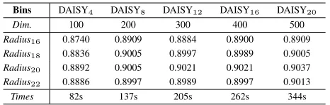
DAISY involves four parameters, radius, the number of ring, the division of sector, and the level of quantization. We set the rings and sectors as 3 and 8, and change the radius and the quantization level. Hessian detector is employed to seek the keypoints. Effect of the parameters on performance are tabu-lated in TABLE IV5. As can be seen, the recognition accuracy has been improved with the number of bins increased. The bigger the number of bins, the better the performance. Mean-while, the dimension of feature is also increased. DAISY20

4_{The source code of AB-SIFT was not available. We implement it by only}

changing the log-polar sector and the level of quantization. In each cell, the generation of histogram is similar to previous work.

5_{DAISY is a dense descriptor to wide-baseline stereo. We first compute the}

descriptors pixel by pixel, and then extract the ones in the site of keypoints. It is detailed in http://cvlab.epfl.ch/∼_tola.

even results in 500-D feature, greatly higher than the preceding descriptors. As for the radius of rings, it is proportional to the recognition accuracy. The longer the radius, the better the performance. The performance reaches a plateau when the radius is beyond 20. To make a balance between efficiency and accuracy, we set the radius as 20, and the number of bins as 8. The running times of different settings are reported. We can see that the computational cost is acceptable.

TABLE IV. THE PERFORMANCE OFDAISYOVER THE RADIUS AND

QUANTIZATION LEVEL.

Bins DAISY4 DAISY8 DAISY12 DAISY16 DAISY20

Dim. 100 200 300 400 500

Radius16 0.8740 0.8909 0.8884 0.8900 0.8909

Radius18 0.8836 0.9005 0.8997 0.8989 0.9005

Radius20 0.8892 0.9005 0.9021 0.9021 0.9037

Radius22 0.8886 0.8997 0.8989 0.8997 0.9013

Times 82s 137s 205s 262s 344s

Fig. 13 compares with all of the local descriptors. Hessian-Laplace and Harris-Hessian-Laplace detectors are employed to search the keypoints. The neighborhood around the detected key-points are characterized by the representative descriptors, SIFT, GLOH, AB-SIFT, DAISY, and SURF6_{. In the prototype of}

SIFT, the neighborhood is quantized into a 4×4 square grids, and the gradient angle is quantized into 8 orientations, resulting in a 128D descriptor. The implementation of GLOH is slightly different from the original work [42]. We assign a log-polar location grid with 3 bins in the radial direction and 8 bins in the angular direction. The central bin is not divided in angular directions. The gradient orientations are further quantized into 8 bins, generating a 17×8=136D feature. SURF quantizes the neighborhood around keypoint into a 4×4 square grids, in each of which four Haar-like wavelet responses are extracted, resulting in a 64D representation.

Harris−Laplace DoG Hessian Hessian−Laplace FAST 0.72

0.74 0.76 0.78 0.8 0.82 0.84 0.86 0.88 0.9 0.92

Detectors

SURF SIFT GLOH ABSIFT DAISY

Fig. 13. Recognition performance obtained using various descriptors.

As can be seen, the recognition performance may be relevant to whatever the keypoint detector is considered. For DoG detector, the performance obtained using DAISY is poorer than SIFT and GLOH. For the remaining detectors, Hessian, Hessian-Laplace, and Harris-Laplace, DAISY outperforms the 6_{The source codes and more details can be found at Chris Evans’s}

(10)

other local features, with a gain greater than 3%∼8% over than SIFT and GLOH. SURF generates the lowest recognition accuracy, even 11.63%, 12.40%, and 15.81% lower than SIFT, GLOH, and DAISY when Hessian detector is employed. This result can be attributed to the fashion of keypoint detection and feature representation. To boost the computational effi-ciency, SURF circumvents image convolutions by means of integral images. Fig. 14 provides a pair of detection maps generated by ‘Fast-Hessian’ and the prototype of Hessian detector. As can be seen, the keypoints detected by ‘Fast-Hessian’ are irregularly scattered in the whole image. Con-trarily, the keypoints produced by Hessian detector are mainly concentrated in target imaging region. They are representative to reflect the target scattering phenomenology. Furthermore, SURF represents the local pattern by the Haar-like wavelet response, hx, hy,|hx|,|hy|, resulting in a 64-D feature. The

discriminative ability is limited in comparison to SIFT, GLOH, and DAISY, whose representations are 128-, 136-, and 200-dimension. The experimental results also prove that the ap-proximation of convolution with integral image is not effective to radar image due to the multiplicative noise.

We can see that AB-SIFT tends to perform better than GLOH, while GLOH always outperforms SIFT. It is not surprising that SIFT performs poorly than GLOH, since GLOH employs a much finer division of location, log-polar sectors. As for the performance rank between DAISY and the remaining descriptors, it depends on the choice of detector. Overall, the combination of FAST detector with DAISY descriptor is the preferable choice in terms of recognition accuracy.

0 20 40 60 80 100

10

20

30

40

50

60

70

80

90

0 20 40 60 80 100

10

20

30

40

50

60

70

80

90

Fig. 14. The detection map produced by ‘Fast-Hessian’ and Hessian detectors. Keypoints defined by ‘Fast-Hessian’ are marked by diamond in yellow, while the ones produced by Hessian are noted by circle in red.

C. Classification

This paper proposes two kinds of methods to target classifi-cation. The effect of related factors on recognition performance is studied. Our first proposed method, sparse representation over neighbor descriptors is abbreviated as NSR.

1) Sparse Representation: Our first proposed scheme refers to building multiple linear regression models. The regression coefficients are obtained according to the thought of sparse representation. Different from the preceding works, where the query (feature) is directly represented by the whole training set (features), this paper develops a prescreener procedure, with which only the nearest neighbor descriptors are kept. The local descriptors far away from the query are ignored. The related factors therefore include the number of neighbor descriptorL

and the regularization parameter λ. To study their effect, we perform two sets of experiments. Hessian detector is used to search keypoints, while SIFT and GLOH are evaluated.

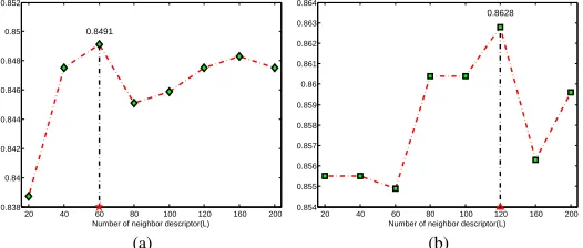
Fig. 15 draws the recognition accuracy across the number of neighbor descriptor (the prescreener). We tune the number of neighbor descriptor from [20, 40, 60, 80, 100, 120, 160, 200]. The recognition accuracies are slightly varied with the number of neighbors changed. For SIFT, the best recognition rate is obtained using sparse representation over 60-nearest-neighbor descriptors, while the best performance for GLOH descriptor is produced by sparse representation over 120-nearest-neighbor descriptors. The recognition performance reaches the plateau when the number of neighbor is bigger than 60 and less than 120. To draw a balance, 120-nearest-neighbor strategy is employed to build a dictionary, over which the descriptors of query can be represented.

20 40 60 80 100 120 160 200

0.838 0.84 0.842 0.844 0.846 0.848 0.85 0.852

Number of neighbor descriptor(L)

0.8491

(a)

20 40 60 80 100 120 160 200

0.854 0.855 0.856 0.857 0.858 0.859 0.86 0.861 0.862 0.863 0.864

Number of neighbor descriptor(L)

0.8628

(b)

Fig. 15. Recognition accuracy across the number of neighbor descriptor. (a) SIFT, (b) GLOH.

Fig. 16 plots the recognition performance as a function of regularization parameter. The results are similar to the above experiments. The recognition accuracy is varied when the regularization parameter is changed. The best recognition rate for SIFT is obtained by 0.18, while the best performance for GLOH is produced by 0.16. The performance is robust for both two descriptors when the parameter value is beyond 0.1 and below 0.2. To obtain a tradoff, this paper set the regularization parameter as 0.18.

0.01 0.05 0.1 0.12 0.16 0.18 0.2

0.834 0.836 0.838 0.84 0.842 0.844 0.846 0.848 0.85

Regulizer(λ)

0.8483

(a)

0.01 0.05 0.1 0.12 0.16 0.18 0.2

0.854 0.855 0.856 0.857 0.858 0.859 0.86 0.861 0.862 0.863 0.864

Regulizer(λ)

0.8628

(b)

Fig. 16. Recognition accuracy across the regularization parameter. (a) SIFT, (b) GLOH. Performance plateaus whenλis bigger than 0.1.

(11)

to define a new single feature. The new defined feature is fed into a trained discriminative classifier. We evaluate several different experimental settings. Hessian detector is used to produce the keypoint, while DAISY descriptor is employed to characterize the local pattern.

BoW.We verify two tricks, LLC [49] and SC [48], popularly studied in the preceding works. We manually change the number of neighbors from 4 to 20 (LLC). The results are displayed in Fig. 17, where the performance obtained using SC is given as the baseline. We can see the recognition performance is changed with the size of codebook increased. For 1024-atom codebook, the recognition accuracy obtained using SC is much better than all settings of LLC. On the contrary, the recognition rate obtained using linear coding is better than sparse coding when 3072-atom codebook is gen-erated. For 2048-atom codebook, the recognition rate for SC is better than LLC(10) and LLC(20), and poorer than LLC(4), LLC(5), LLC(6), and LLC(8). The recognition performance is proportional to the size of codebook. For locality-constrained linear coding, the number of neighbors plays an important role. The little neighbor (5) produces the better performance. In addition, linear coding is computationally more attractive than sparse coding.

1024 2048 3072 0.86

0.87 0.88 0.89 0.9 0.91

0.92 LLC(4) LLC(5) LLC(6) LLC(8) LLC(10) LLC(20) SC(1024) SC(2048) SC(3072)

Fig. 17. Performance obtained using LLC and SC.

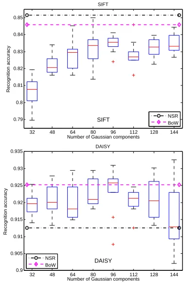
FV.Fisher vectors approximates the distribution of low-level features with Gaussian mixture model. The related factor to be decided is the number of Gaussian components. We change the number of Gaussian components from 32 to 144. Since the parameters, mean, covariance, and prior are randomly initialized, the recognition accuracies are not deterministic. We implement FV with the same setting repeatedly for 10 times. The recognition performance as a function of the number of Gaussian components is shown in Fig. 18, in which NSR and BoW are employed as the baseline. Two descriptors, SIFT and DAISY are assessed. We found the recognition performance is different for two descriptors when the number of Gaussian components is changed. For SIFT, FVs with all of Gaussian components perform poorly than NSR and BoW. FV with 96-Gaussian-component produces the better and robust performance. For DAISY, most settings of FV perform better than NSR, and poor than BoW with 3072-atom-codebook. Again, FV with 96-Gaussian-component achieves the better

and robust performance than the remaining settings.

32 48 64 80 96 112 128 144 0.79

0.8 0.81 0.82 0.83 0.84 0.85

Number of Gaussian components

SIFT

SIFT NSR

BoW

32 48 64 80 96 112 128 144 0.9

0.905 0.91 0.915 0.92 0.925 0.93 0.935

Number of Gaussian components

DAISY

NSR BoW

Fig. 18. Recognition accuracy of FV across the number of Gaussian components. Performance plateaus whenλis bigger than 0.1.

The experimental results prove that 120-nearest-neighbor is appropriate for NSR, while 2048- and 3072-atom-codebook is suitable for BoW. NSR and BoW are the preferable classifier for SIFT, GLOH, and AB-SIFT, while FV is more appropriate for DAISY.

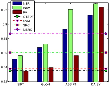
D. The Validation of Recognition Performance

This paper achieves radar target recognition by keypoint-based local descriptor. Two kinds of methods are proposed to implement classification. The effect of related factors are studied previously. The recognition performance of proposed strategy is validated. State-of-the-art global features are em-ployed as the baseline. Support vector machine learning (SVM) is popularly studied over the years [7]. Sparse representation-based classification (SRC) is a recently developed method [8], [32]. Both of them input the raw pixel values for classifi-cation7. Furthermore, the preceding works achieve distortion and translation invariance by Fourier transformed spectrum. The representative includes optional tradeoff synthetic dis-criminant function (OTSDF) [52]. Another family of filter banks, the monogenic signal, has also been used for target classification [14]–[16] (MSRC). These methods are employed

7_{The feature dimension is reduced by downsampling, principal component}

(12)

to compared with the proposed strategy. The experimental results are given in Fig. 19.

SIFT GLOH ABSIFT DAISY 0.82

0.84 0.86 0.88 0.9 0.92

NSR BoW FV OTSDF SVM SRC MSRC

Fig. 19. Comparison to the preceding works.

From Fig. 19, we found the recognition performance ob-tained using four kinds of local descriptors are sharply differ-ent. For SIFT, GLOH, and AB-SIFT, NSR performs better than FV, and poorly than BoW. Differently, the recognition accuracy obtained using FV with DAISY is better than NSR, and poorly than BoW. On the other hand, DAISY with NSR, BoW, and FV, outperforms all baseline algorithms, even 2.57%, 3.85%, and 3.79% better than the main competitor, MSRC. Similarly, AB-SIFT with NSR and BoW also performs better than the baselines. The performance obtained by SIFT is poor than SRC and MSRC, and better than SVM and OTSDF. The recognition accuracy for GLOH is poorer than MSRC, and better than SVM, SRC, and OTSDF. The results prove that the local descriptor could achieve comparable or even better performance compared to the global feature.

V. CONCLUSION

This paper considers radar target recognition with keypoint-based local descriptor. We develop two kinds of schemes to implement classification. Multiple comparative experiments are performed, from which several different combinations of detectors and descriptors are evaluated. The experimental results prove:

• keypoint-based local descriptor could be fully tuned to target recognition,

• it is important to configure the related factors appropri-ately,

• the proposed strategy could achieve comparable or even better performance than the preceding studies,

• the proposed strategy provides great potential for target recognition under the non-literal conditions,

• the local descriptors can be further refined according to the imaging mechanism of radar.

However, some issues are needed to be further considered. We plan to study whether the advantage of our proposed strategy will persist under the non-literal conditions.

We design a prescreener procedure for sparse representation. It makes the computational cost and memory consumption

acceptable. The linear correlation response is employed to measure the (dis)similarity. An important future research di-rection is to develop the specific metric. The study on the measurement of similarity has been noticed in [53], [54] and more recently explored in [55]. The further research in target recognition is yet to be uncovered.

On the other hand, this paper verifies the generic model of local descriptor by some fundamental experiments. The mech-anism of radar imaging is not yet considered in the phase of detection, or representation. We believe the performance can be improved if the specificity of SAR image has been exploited. Moreover, addressing the problem of target recognition under the less constrained conditions is another interesting direction for future work.

REFERENCES

[1] L. Potter and R. Moses, “Attributed scattering centers for SAR ATR,” IEEE Trans. Image Process., vol. 6, no. 1, pp. 79–91, Jan. 1997. [2] C. Olson and D. Huttenlocher, “Automatic target recognition by

match-ing oriented edge pixels,”IEEE Trans. Image Process., vol. 6, no. 1, pp. 103–113, Jan. 1997.

[3] L. Novak, G. Owirka, and C. Netishen, “Performance of a high-resolution polarimetric SAR automatic target recognition system,” Lin-coln Lab J., vol. 6, no. 1, pp. 11–23, 1993.

[4] A. Banerjee, P. Burlina, and R. Chellappa, “Adaptive target detection in foliage-penetrating SAR images using alpha-stable models,” IEEE Trans. Image Process., vol. 8, no. 12, pp. 1823–1831, Dec. 1999. [5] D. Kreithen, S. Halversen, and G. Owirka, “Discriminating targets from

clutter,”Lincoln Lab J., vol. 6, no. 1, pp. 25–52, 1993.

[6] L. Novak, G. Owirka, and A. Weaver, “Automatic target recognition using enhanced resolution SAR data,”IEEE Trans. Aerosp. Electron. Syst., vol. 35, pp. 267–278, 1999.

[7] Q. Zhao and J. Principe, “Support vector machines for SAR automatic target recognition,”IEEE Trans. Aerosp. Electron. Syst., vol. 37, no. 2, pp. 643–654, Apr. 2001.

[8] J. Thiagarajan, N. Karthikeyan, K. Peter, P. Knee, A. Spanias, and V. Berisha, “Sparse representation for automatic target classification in SAR images,” in Int’l Sym. Communcitaion, Control and Signal Processing, 2010, pp. 1–4.

[9] M. Liu, Y. Wu, P. Zhang, Q. Zhang, Y. Li, and M. Li, “SAR target con-figuration recognition using locality preserving property and gaussian mixture distribution,”IEEE Geosci. Remote Sens. Lett., vol. 10, no. 2, pp. 268–272, Mar. 2013.

[10] X. Huang, H. Qiao, and B. Zhang, “SAR target configuration recog-nition using tensor global and local discriminant embedding,” IEEE Geosci. Remote Sens. Lett., vol. 13, no. 2, pp. 222–226, Feb. 2016. [11] Z. Cui, Z. Cao, J. Yang, J. Feng, and H. Ren, “Target recognition in

synthetic aperture radar images via non-negative matrix factorisation,” IET Radar, Sonar & Navigation, vol. 9, no. 9, pp. 1376–1385, Dec. 2015.

[12] R. Patnaik and D. Casasent, “MINACE filter classification algorithms for ATR using MSTAR data,” inAutomatic Target Recognition XV, Proc. SPIE, vol. 5807, Aug. 2005, pp. 100–111.

[13] ——, “MSTAR object classification and confuser and clutter rejection using MINACE filters,” in Automatic Target Recognition XVI, SPIE, vol. 6234, Aug. 2006, pp. 1–13.

[14] G. Dong, N. Wang, and G. Kuang, “Sparse representation of monogenic signal: with application to target recognition in SAR images,” IEEE Signal Process. Lett., vol. 21, no. 8, pp. 952–956, Aug. 2014. [15] G. Dong and G. Kuang, “Classification on the monogenic scale space:

(13)

[16] G. Dong, G. Kuang, N. Wang, and W. Wang, “Classification via sparse representation of steerable wavelet frames on grassmann manifold: Application to target recognition in SAR image,”IEEE Trans. Image Process., vol. 26, no. 6, pp. 2892–2904, Jun. 2017.

[17] M. Felsberg and G. Sommer, “The monogenic signal,” IEEE Trans. Signal Process., vol. 49, no. 12, pp. 3136–3144, 2001.

[18] ——, “The monogenic scale-space: A unifying approach to phase-based image processing in scale space,”J. Math. Imag. Vis., vol. 21, no. 1, pp. 5–26, 2004.

[19] J. Park, S. Park, and K. Kim, “New discrimination features for SAR automatic target recognition,”IEEE Geosci. Remote Sens. Lett., vol. 10, no. 3, pp. 476–480, May 2013.

[20] J. Zhu, X. Qiu, Z. Pan, Y. Zhang, and B. Lei, “An improved shape contexts based ship classification in SAR images,” Remote Sensing, vol. 9, no. 2, 2017.

[21] J. Singh and M. Datcu, “SAR image categorization with log cumulants of the fractional Fourier transform coefficients,”IEEE Trans. Geosci. Remote Sens., vol. 51, no. 12, pp. 5273–5282, Dec. 2013.

[22] M. Amoon and G.-A. Rezai-rad, “Automatic target recognition of synthetic aperture radar (SAR) images based on optimal selection of Zernike moments features,”IET Computer Vision, vol. 8, pp. 77–85, 2014.

[23] X. Zhang, Z. Liu, S. Liu, D. Li, Y. Jia, and P. Huang, “Sparse coding of 2D-slice Zernike moments for SAR ATR,”International Journal of Remote Sensing, vol. 38, pp. 412–431, 2016.

[24] P. Bolourchi, H. Demirel, and S. Uysal, “Target recognition in sar images using radial Chebyshev moments,” Signal Image & Video Processing, vol. 11, p. 10331040, 2017.

[25] S. Chen, H. Wang, F. Xu, and Y.-Q. Jin, “Target classification using the deep convolutional networks for SAR images,”IEEE Trans. Geosci. Remote Sens., vol. 54, no. 8, pp. 4806–4817, Aug. 2016.

[26] J. Ding, B. Chen, H. Liu, and M. Huang, “Convolutional neural network with data augmentation for SAR target recognition,” IEEE Geosci. Remote Sens. Lett., vol. 13, no. 3, pp. 364–368, March 2016. [27] N. Wang, Y. Wang, H. Liu, Q. Zuo, and J. He, “Feature-fused SAR

target discrimination using multiple convolutional neural networks,” IEEE Geosci. Remote Sens. Lett., vol. 14, no. 10, pp. 1695–1699, Oct. 2017.

[28] D. Malmgren-Hansen, A. Kusk, J. Dall, A. A. Nielsen, R. Engholm, and H. Skriver, “Improving SAR automatic target recognition models with transfer learning from simulated data,”IEEE Geosci. Remote Sens. Lett., vol. 14, no. 9, pp. 1484–1488, Sept. 2017.

[29] S. Deng, L. Du, C. Li, J. Ding, and H. Liu, “SAR automatic target recognition based on Euclidean distance restricted autoencoder,”IEEE J. Sel. Topics Appl. Earth Observ. Remote Sens., vol. 10, no. 7, pp. 3323–3333, Jul. 2017.

[30] B. Ding, G. Wen, X. Huang, C. Ma, and X. Yang, “Target recognition in synthetic aperture radar images via matching of attributed scattering centers,”IEEE J. Sel. Topics Appl. Earth Observ. Remote Sens., vol. 10, no. 7, pp. 3334–3347, July 2017.

[31] L. Novak, G. Owirka, and W. Brower, “Performance of 10- and 20-target MSE classifiers,” IEEE Trans. Aerosp. Electron. Syst., vol. 36, pp. 1279–1289, Oct. 2000.

[32] J. Wright, A. Yang, A. Ganesh, S. Sastry, and Y. Ma, “Robust face recognition via sparse representation,”IEEE Trans. Pattern Anal. Mach. Intell., vol. 31, no. 2, pp. 210–227, Feb. 2009.

[33] D. Lowe, “Distinctive image features from scale-invariant keypoints,” Int’l J. Comput. Vis., vol. 60, no. 2, pp. 91–110, Nov. 2004. [34] C. Harris and M. Stephen, “A combined corner and edge detector,” p.

10.5277, Aug. 1988.

[35] T. Lindeberg, “Feature detection with automatic scale selection,”Int’l J. Comput. Vis., vol. 30, no. 2, pp. 79–116, 1998.

[36] K. Mikolajczyk and C. Schmid, “Scale & affine invariant interest point detectors,”Int’l J. Comput. Vis., vol. 60, no. 1, pp. 63–86, 2004.

[37] H. Bay, T. Tuytelaars, and L. V. Gool, “Surf: Speeded up robust features,” inProc. Eur. Conf. Comput. Vis., 2006, pp. 404–417. [38] H. Bay, A. Ess, T. Tuytelaars, and L. V. Gool, “Speeded-up robust

features (SURF),”Computer Vision and Image Understanding, vol. 110, no. 3, pp. 346–359, 2008.

[39] E. Rosten and T. Drummond, “Machine learning for high-speed corner detection,” inProc. Eur. Conf. Comput. Vis., 2006, pp. 430–443. [40] E. Rosten, R. Porer, and T. Drummond, “Faster and better: A machine

learning approach to corner detection,”IEEE Trans. Pattern Anal. Mach. Intell., vol. 32, no. 1, pp. 105–119, Jan 2010.

[41] D. Lowe, “Object recognition from local scale-invariant features,” in Proc. IEEE Int’l Conf. Comput. Vis. (ICCV), 1999, pp. 1150–1157. [42] K. Mikolajczyk and C. Schmid, “A performance evaluation of local

descriptors,”IEEE Trans. Pattern Anal. Mach. Intell., vol. 27, no. 10, pp. 1615–1630, Oct. 2005.

[43] A. Sedaghat and H. Ebadi, “Remote sensing image matching based on adaptive binning SIFT descriptor,”IEEE Trans. Geosci. Remote Sens., vol. 53, no. 10, pp. 5283–5293, Oct. 2015.

[44] E. Tola, V. Lepetit, and P. Fua, “A fast local descriptor for dense matching,” inProc. IEEE Conf. Comput. Vis. Pattern Recognit., 2008, pp. 1–8.

[45] ——, “DAISY: An efficient dense descriptor applied to wide-baseline stereo,” IEEE Trans. Pattern Anal. Mach. Intell., vol. 32, no. 5, pp. 815–830, May 2010.

[46] E. Candes and T. Tao, “Near-optimal signal recovery from random projections: Universal encoding strategies,” IEEE Trans. Inf. Theory, vol. 52, no. 12, pp. 5406–5425, 2006.

[47] S. Lazebnik, C. Schmid, and J. Ponce, “Beyond bags of features: Spatial pyramid matching for recognizing natural scene categories,” in Proc. IEEE Conf. Comput. Vis. Pattern Recognit., 2006, pp. 2169–2178. [48] J. Yang, K. Yu, Y. Gong, and T. Huang, “Linear spatial pyramid

matching using sparse coding for image classification,” inProc. IEEE Conf. Comput. Vis. Pattern Recognit., Jun. 2009, pp. 1794–1801. [49] J. Wang, J. Yang, K. Yu, F. Lv, T. Huang, and Y. Gong,

“Locality-constraint linear coding for image classification,” inProc. IEEE Conf. Comput. Vis. Pattern Recognit., Jun. 2010, pp. 3360–3367.

[50] F. Perronnin and C. Dance, “Fisher kernels on visual vocabularies for image categorization,” in Proc. IEEE Conf. Comput. Vis. Pattern Recognit., June 2007, pp. 1–8.

[51] F. Perronnin, J. Snchez, and T. Mensink, “Improving the Fisher kernel for large-scale image classification,” inProc. Eur. Conf. Comput. Vis., 2010, pp. 1–14.

[52] R. Singh and B. Kumar, “Performance of the extended maximum average correlation height filter and the polynomial distance classifier correlation filter for multiclass SAR detection and classification,” in Algorithms for SAR Imagery IX, vol. 4727. SPIE, 2002, pp. 265–279. [53] E. Levina and P. Bickel, “The Earth Mover’s distance is the mallows distance: Some insights from statistics,” in Proc. IEEE Int’l Conf. Comput. Vis. (ICCV), 2001, pp. 251–256.

[54] Y. Rubner, C. Tomasi, and L. Guibas, “The Earth Mover’s distance as a metric for image retrieval,”Int’l J. Comput. Vis., vol. 40, no. 2, pp. 99–121, 2000.