Mixed Burr Type X Distribution under Type I Censored Samples
Tabassum Naz Sindhu
Department of Statistics
Quaid-i-Azam University 45320, Islamabad 44000, Pakistan [email protected]
Navid Feroze
Department of Mathematics and Statistics
Allama Iqbal Open University, Islamabad, Pakistan [email protected]
Muhammad Aslam
Department of Statistics
Quaid-i-Azam University 45320, Islamabad 44000, Pakistan [email protected]
Abstract
The paper is concerned with the preference of prior for the Bayesian analysis of the shape parameter of the mixture of Burr type X distribution using the censored data. We modeled the heterogeneous population using two components mixture of the Burr type X distribution. A comprehensive simulation scheme, through probabilistic mixing, has been followed to highlight the properties and behavior of the estimates in terms of sample size, corresponding risks and the proportion of the component of the mixture. The Bayes estimators of the parameters have been evaluated under the assumption of informative and non-informative priors using symmetric and asymmetric loss functions. The model selection criterion for the preference of the prior has been introduced. The hazard rate function of the mixture distribution has been discussed. The Bayes estimates under exponential prior and precautionary loss function exhibit the minimum posterior risks with some exceptions.
Keywords: Inverse Transformation Method, Loss Functions, Prior Predictive distributions, Credible Intervals.
1. Introduction
Burr (1942) introduced twelve different forms of cumulative distribution functions for modeling lifetime data. Among those twelve distribution functions, Burr-Type X and Burr-Type XII have received the maximum attention. Surles and Padgett (2001) observed that the Burr-Type X distribution can be used quite effectively in modeling strength data and general lifetime data. Several aspects of the one-parameter (Scale = 1) Burr-Type X distribution have been studied by Sartawi and Abu-Salih (1991), Jaheen (1996), Ahmad et al. (1997) and Raqab (1998). The distribution function and the density function of a Burr-Type X distribution have closed form. As a consequence of that, it can be used very conveniently even for censored data.
Demidenko (2004), Sultan et al. (2007), Nair and Abdul (2010), Afify (2011) and Erisoglu et al. (2011). Gosh and Ebrahimi (2001) have made the Bayesian analysis of the mixing function in a mixture of two exponential distributions. Saleem and Aslam (2008) presented a comparison of the Maximum Likelihood (ML) estimates with the Bayes estimates assuming the uniform and the Jeffreys priors for the parameters of the Rayleigh mixture. Saleem et al. (2010) considered the Bayesian analysis of the mixture of Power function distribution using the complete and the censored sample.
The problem of censoring is more commonly encountered in life-time data because no experiment may remain sustained for an infinite time due to restrictions on the available time or cost for testing. There are different kinds of censoring schemes which include right, left and interval censoring, single or multiple censoring and type-I or type-II censoring. Type-I and type-II censoring schemes are most popular among them. Saleem et al.(2010) considered the Bayesian analysis of the power function mixture distribution using type-I censored data. Shi and Yan (2010) discussed the empirical Bayes estimates of two-parameter exponential distribution under type-I censoring.
We have focused on the selection of suitable prior for Bayesian analysis of the mixture of Burr type X distribution under type I censored samples. It worth mentioning here, that the mixture of this model under Bayesian approach has not been considered in the literature yet.
The article is outlined as follows. In the section 2, we defined the mixture model for Burr type X distribution, sampling and likelihood function for type I censored samples. In the section 3, the posterior distributions have been derived under different priors. The loss functions for the derivation of Bayes estimators and posterior risks have been introduced in the section 4. Method of elicitation of hyper-parameters for the mixture of Burr type X distribution via prior predictive approach has been discussed in the section 5. Credible intervals for the parameters of the model have been derived in the section 6. The posterior predictive distributions have been presented in the section 7. A simulation study along with graphical representation of the results has been performed in the section 8. A real life example has been included in the section 9. The section 10 contains the discussion regarding the hazard rate function of the mixture model. The model selection criterion has been introduced in the section 11. The section 12 presents the conclusion of the study.
2. The Population and the Model
2
11( ) 1
F x exp x and F x2( )
1 exp
x2
2. The corresponding finite mixture density function has its probability density function (pdf) as:
2
2
1 1
2
2
2 11 2 1 2
( , , ) 2 exp 1 exp (1 )2 exp 1 exp ,
p x w w x x x w x x x
|
0, 1, 2; 0
i i x
(1)
The graphs of the mixture model, given in (1), are presented in the following. The abbreviations used in the legends are: PR1: λ1 = 1.50, λ 2 = 0.75; PR2: λ1 = 2.75, λ2 = 2.00;
PR3: λ1 = 3.50, λ2 = 3.00; PR4: λ1 = 4.50, λ2 = 4.00; PR11: λ1 = 0.50, λ2 = 0.75; PR12:
λ1 = 2.75, λ2 = 4.50; PR13: λ1 = 3.50, λ2 = 5.00; PR14: λ1 = 4.50, λ2 = 6.00.
From the graphs it can be seen that the mixture model shifts its origin to the right for larger values of the parameters. In addition, the larger values of the parameters decrease the spread and increase the height of the curves.
Fig. 1: Graph of the mixture model using π = 0.25 Fig. 2: Graph of the mixture model using π = 0.75
Fig. 3: Graph of the mixture model using π = 0.25 Fig. 4: Graph of the mixture model using π = 0.75
0.5 1.0 1.5 2.0 2.5 3.0 x
0.2 0.4 0.6 0.8 1.0 f x
P R4 P R3 P R2 P R1 Curves
0.5 1.0 1.5 2.0 2.5 3.0 x
0.2 0.4 0.6 0.8 1.0 f x
P R4 P R3 P R2 P R1 Curves
0.5 1.0 1.5 2.0 2.5 3.0 x
0.2 0.4 0.6 0.8 1.0 f x
P R14 P R13 P R12 P R11 Curves
0.5 1.0 1.5 2.0 2.5 3.0 x
0.2 0.4 0.6 0.8 1.0 f x
2.1. Sampling
A random sample of size n units from the above mixture model is operating to a life testing experiment. The test is terminated at a fixed time T. Let the test be conducted and it is observed that out of n, r units have lifetime in the interval
0,T and
nr
units are still functioning when the test termination time T is over. Hence
nr
units that have not failed by the time T are censored objects and yield no information. According to Mendenhall and Hader (1958), in many real life situations only the failed objects can easily be identified as member of either subpopulation 1 or subpopulation 2. So, depending upon the cause of failure it may be observed that r1and r2 objects are identified as members of the first subpopulation and the second subpopulation respectively. Obviously r r1 r2 and remaining
nr
units provide no information about the subpopulation to which they belong. Furthermore, let xijas the failure time of the jth unit to the ith subpopulation, where j1, 2,..., ,r ii 1, 2;0x1j,x2j T.2.2. The Maximum Likelihood Function
The likelihood function for a two-component mixture with n items under study, the probability that r1 will fail due to cause 1, r2 will fail due to cause 2 and remaining
1 2
(n r r ) will survive at time T when test is terminated is given as:
1 2
1 2 1 1 2 2
1 1
( , , x) 1 1
r r
n r
j j
j j
L w wf x w f x F T
1 21 2 2 1 2 2 2 1
1 2 1 1 1 1 1 1 2 2 2 2
1 1
2 2
1 2
, , x 2 exp 1 exp (1 )2 exp 1 exp
1 exp ln 1 exp 1 exp ln 1 exp
r r
j j j j j j
j j
n r
L w w x x x w x x x
w T w T
| 1
1 2 1 1 2 2
1 2
2
1 1 2
0 0 1 1 2
, , x 1 1 iexp
n r k n r
k k r k r k r
i i ij ij
k k i
n r n r k
L w w w x
k k
| (2) where 1 211 12 1 21 22 2 ( , ) (x ,x ,...,xr,x ,x ,...,x r ) 1 2
x x x is data,
1
1
12 2
1 1 1 1
1
ln 1 exp ln 1 exp
r
j j j
j
x x k T
and
2 1 1
2 2
2 2 2 2
1
ln 1 exp ln 1 exp
r
j j j
j
x x k T
3. Prior and Posterior Distributions
observations supposed to be added to the given sample size. While, when significant information is not avaiable regarding the parameters of the sampling distribution, a non-informative prior can be formed. We have assumed both non-informative and non-non-informative priors for the posterior estimation.
3. 1. Posterior Distribution under Uniform Prior
Let us assume a state of ignorance that 1, 2and ware uniformly distributed over(0, ) . Hence
1( )1 1, 2( 2) 2, i 0
p k p k p w3( )1, i1, 2, 0 w 1 (3)
Assuming independence, we have an improper joint prior that is proportional to a constant. The joint prior is incorporated with the likelihood (2) to yield a proper joint posterior distribution of 1, 2 and .w The joint posterior distribution of 1, 2 and wis
1
1 2 1 1 2 2
1 2
2
1
1 2
0 0 1 1 2
1 1
( , , x 1 1 iexp
n r k n r
k k r k r k r
i i ij ij k k i
k
n r n r k
p w w w x
k k
| ) 0, i 0 w 1 (4)
where 1 r1 k1 1, 2 r2 k2 1,B
1, 2
is a standard beta function and 1kisdefined as:
1 1 2 1 2 1 21 1 2
1 1 2 1 1
0 0 1 2
1 1 2 2
1 1
1 ,
n r k n r
k k
k r r
k k
j j j j
n r n r k r r
B
k k x x
3. 2. Posterior Distribution under Jeffreys Prior
Jeffreys prior is locally uniform and hence non-informative. An appealing property of Jeffreys prior is that it is invariant with respect to one-to-one transformations. For the Burr type x model given in Section 2, the Jeffreys priors are p1( )1 11, 01 ,
2 2 2
1 2
( ) , 0
p andp w3( )1, 0 w 1. assuming independence, the joint prior
2
1
1 1 2
( , , )
g w is incorporated with the likelihood (2) to yield a proper joint posterior distribution of 1, 2and w.Thejoint posterior distribution under Jeffreys prior is:
1
1 2 1 1 2 2
1 2
2
1 1
1 2
0 0 1 1 2
2 1
( , , x 1 1 i exp
n r k n r
k k r k r k r
i i ij ij
k k i k
n r n r k
p w w w x
k k
| ) 0, i 0 w 1 (5)
where 2k is defined as:
1 1 2 1 2 1 21 1 2
2 1 2
0 0 1 2
1 1 2 2
1 , .
n r k n r
k k
k r r
k k
j j j j
n r n r k r r
B
k k x x
3.3. Posterior Distribution under Gamma Prior
In case of an informative prior, the use of prior information is equivalent to add a number of observations to the given sample size and hence leads to a reduction of posterior risks of the Bayes estimates based on the said informative prior.
Let
1 Gamma a b
1, 1
, 2 Gamma a b
2, 2
are the gamma priors and ( )p w3 1,, 0,
i i
a b i1, 2, 0 w 1
Assuming independence, the joint prior is incorporated with the likelihood to give the joint posterior distribution, that is
1 1 1 2 2 1
1 2 1 2 1 1 2 2
( , , r a r a exp exp
p w) b b . The joint posterior distribution of 1, 2
and wis
1
1 2 1 1 2 2
1 2
2
1 1
1 2
0 0 1 1 2
3
1
( , , x 1 1 i i exp
n r k n r
k k r k r k r a
i i i ij ij
k k i
k
n r n r k
p w w w b x
k k
| ) 0, i 0 w 1 (6)
where 3k is defined as:
1 1 21 1 2 2
1 2
1 1 1 2 2
3 1 2
0 0 1 2
1 1 1 2 2 2
1 ,
n r k n r
k k
k r a r a
k k
j j j j
n r n r k r a r a
B
k k b x b x
3.4. Posterior Distribution under Exponential Prior
Let
1 Exp
1 , 2 Exp
2 are the exponential priors and p w3( )1, i 0,1, 2, 0 1
i w
Assuming independence, the joint prior is incorporated with the likelihood to give the joint posterior distribution, that is
1 2 1 1 2 2
( , , exp exp
p w) . The joint posterior distribution of 1, 2and wis
1
1 2 1 1 2 2
1 2
2
1
1 2
0 0 1 1 2
4
1
( , , x 1 1 iexp
n r k n r
k k r k r k r
i i i ij ij
k k i
k
n r n r k
p w w w x
k k
| ) 0, i 0 w 1 (7)
where 4k is defined as:
1 1 2 1 2 1 21 1 2
4 1 2 1 1
0 0 1 2
1 1 1 2 2 2
1 1
1 , .
n r k n r
k k
k r r
k k
j j j j
n r n r k r r
B
k k x x
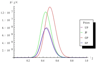
The graphs for the marginal posterior distributions for the parameters of the mixture density, given in (3), (5), (6) and (7) under different priors are presented in the following. The graphs are based on the simulated data from the mixture model using a sample of size 50. The legends in the graphs contain following abbreviations: UP: Uniform prior; JP: Jeffreys prior; GP: Improved gamma prior; EP: Exponential prior.
Fig. 5: Graph of the marginal posterior distribution of λ1 under different priors
Fig. 6: Graph of the marginal posterior distribution of λ2 under different priors
The graphs indicate that the marginal posterior distributions for the parameters λ1 and λ2
are slightly positively skewed. In case of first component, it can be observed that shape of posterior distribution under all the prior are close to each other with slightly different origins. In case of second component, the curves of the posterior distributions under uniform and exponential priors are similar, while the shapes of posterior distributions under Jeffreys and gamma priors are different.
4. Loss Function
The squared error loss function (SELF) is the commonly chosen loss function for the estimation of the parameter. The squared error loss function L
,
2 was proposed by Legendre (1805) and Gauss (1810). This loss function is broadly used because it gives apparently sound Bayesian solution, i.e., those one would usually suggest as estimators for a non-decision theoretic inference based on the posterior distribution. A very useful and simple asymmetric precautionary loss function (PLF) is:* 2
*
*
( )
( , ) .
L
The Bayes estimator and the posterior risk under PLF are
2E
x x and
2
( ( , ) 2
Ex L d Ex x Ex x respectively. The Bayes
estimators are also evaluated under weighted squared error loss function (WSELF). The Bayes estimator and the posterior risk under WSELF are
E
1
1
x x and
1
* 1
( ( , ) .
E L E E
x x x x x Hence, we consider symmetric as well as
asymmetric loss functions for getting better understanding in our Bayesian analysis.
0.05 0.10 0.15 0.20 1
10 20 30 40 p 1 x
EP GP JP UP P riors
0.2 0.4 0.6 0.8 1.0 2
2. 10 8 4. 10 8 6. 10 8 8. 10 8 1. 10 7 1.2 10 7
p 2 x
5. Elicitation of Hyper-parameters of Informative Prior through Prior Predictive Probabilities
To elicit a prior density, Aslam (2003) forms some new methods base on the prior predictive distribution. For the elicitation of hyper-parameters, he considers prior predictive probabilities, predictive mode and confidence level. In this study, the method of prior predictive probabilities is used for obtaining the hyper-parameters of the considered informative prior. In fact, prior predictive removes the uncertainty in parameter (s) to reveal a distribution for the data point only. We suppose that prior predictive probabilities satisfy the laws of probability because this law ensure the expert would be consistent in eliciting the probabilities and some inconsistencies may arise which are not very serious.
A function
a b, is defined in such a way that the hyper-parameters a and b are to bechosen by minimizing this
2 0
,
,
min
a b y
p y p y a b
p y
, where p y
denote the priorpredictive probabilities characterized by the hyper-parameters a and b and p0
ydenote the elicited prior predictive probabilities. The above equations solved simultaneously by applying ‘PROC SYSLIN’ of the SAS package for eliciting the required hyper-parameters.
5.1. Elicitation of hyper-parameters of Gamma Prior
The equation of prior predictive under the gamma prior is given as: 1
1 2 1 2 1 2
0 0 0
( ) ( , , ) ( , , )
p y p w p y w dwd d
| (8)1 2
1 1 1 1 2 1 2 2
1 2
1 2 1 2
1 2
where ( , , )
( ) ( )
a a
a b a b
b b
p w e e
a a
2
2
1 1
2
2
2 11 2 1 2
( , , ) 2 exp 1 exp (1 )2 exp 1 exp
p y| w w y y y w y y y
After some algebra
1 2
1 2
1 1 2 2
1 1
1 1
2 2
1 2
1
2 2
( )
ln 1 exp ln 1 exp
exp 1 exp ,
a a
a a
a b a b
p y
b y b y
y y y
0 y (9)
5.2. Elicitation of hyper-parameters of Exponential Prior
The equation of prior predictive under the exponential prior is given as: 1
1 2 1 2 1 2
0 0 0
( ) ( , , ) ( , , )
p y p w p y w dwd d
|1 1 2 2
1 2 1 2
where ( ,p , )w e e
2
2
1 1
2
2
2 11 2 1 2
( , , ) 2 exp 1 exp (1 )2 exp 1 exp
p y| w w y y y w y y y
After some simplifications the prior predictive distribution becomes:
1
2
1
22 2
1
2 2 1 2
1 2
( )
ln 1 exp ln 1 exp
exp 1 exp ,
p y
y y
y y y
0 y (10)
By using the method of elicitation, mentioned above, we get the following hyper-parametric values 1 0.925806, 2 1.023728.
6. Credible Interval
The Bayesian counterpart of the confidence interval is named as credible interval. Unlike classical confidence interval, the 95% Bayesian credible interval contains the true parameter value with approximately 95% confidence. The credible interval is defined as:
Let p
x
be the posterior distribution; then a 100 1
% credible interval for parameter , in any set C is such that Pp x
C 1 . According to Eberly andCasella (2003) the credible interval can also be defined as:
0 2
x
L
p d
,
x 2U
p d
where L and U are the lower and upper limits of the credible interval respectively and is level of significance.7. Posterior Predictive Distributions
The predictive distribution contains the information about the independent future random observation given preceding observations. In context of Bayesian inference the predictive distribution is referred as the posterior predictive distribution. Bolstad (2004) and Bansal (2007) have given a detailed discussion about the posterior predictive distribution. The posterior predictive distribution can be defined as:
1 1 2
1 2
1 2 0 0 0( , , ) ; , ,
x
x
g y h w f y w dwd d
where h( , 1 2,w
x
)is the posterior mixture distribution, f y
; , 1 2,w
is mixture density for future observation and y = xn+1 is the future observation given the sampleinformation x = x1, x2, ..., xn, from of the model (1). The posterior predictive distribution
using (1) and (12) can be obtained as:
The posterior predictive distribution under uniform prior is:
2 1 1 2 2 1 22 2 1 2
1 2
1 1 2 1 2 1 2 1 2
1 2 2 1 1 2
0 0 1 2
1
1 1 2 2 1 1 2 2
1, 2 1 , 1 1 2
1
( , , x 1
1 ln 1 ln 1
n r k y
n r
k k
r r
y r r
y y
k k k
j j j j j j j j
n r n r k e B r r B r r
p w
k k e x e x x x e
| )
The posterior predictive distribution under Jeffreys prior is:
2 1 1 2 2 1 22 2 1 2
1 2
1 1 2 1 2 1 2 1 2
1 2 1 1
0 0 1 2
1
1 1 2 2 1 1 2 2
1, 1 , 1 1
1
( , , x 1
1 ln 1 ln 1
n r k y
n r
k k
r r
y r r
y y
k k k
j j j j j j j j
n r n r k e B r r B r r
p w
k k e x e x x x e
| )
The posterior predictive distribution under gamma prior is:
2 1 1 2
2 2 1 1 2 2 1 1 2 2 2
1 2
1 1 2 1 1 2 2 1 2 1 1 2 2
1 2 1
0 0 1 2
1
1 1 1 2 2 2 1 1 1 2 2 2
1, 1 , 1 1
1
( , , x 1
1 ln 1 ln 1
n r k y
n r kk
ra r a
y r a ra
y y
k k k
j j j j j j j j
n r n r k e B r a r a B r a r a
p w
k k e x b e x b x b x b e
| ) 1
The posterior predictive distribution under exponential prior is:
2 1 1 2 2 1 22 2 1 2
1 2
1 1 2 1 2 1 2 1 2
1 2 2 1 1 2
0 0 1 2
1
1 1 1 2 2 2 1 1 1 2 2 2
1, 2 1 , 1 1 2
1
( , , x 1
1 ln 1 ln 1
n r k y
n r
k k
r r
y y r r y
k k k
j j j j j j j j
n r n r k e B r r B r r
p w
k k e x v e x v x v x v e
| )
8. Simulation Study
A simulation study is carried out in order to investigate the performance of Bayes estimators and impact of sample size and mixing proportion in the fit of model. We take random samples of sizes n = 25, 50, 100 and 300 from the two component mixture of Burr type x distribution with( , 1 2)
3, 7 , 9, 11
,w0.35. To generate a mixture datawe make use of probabilistic mixing with probability wand(1w). A uniform number u
Table 1: Bayes Estimates (Uniform) of Burr Type X mixture parameters under SELF
n 13 27 w0.35 19 211 w0.35
25 3.84830 7.90969 0.368222 11.29690 12.5169 0.376611 (1.70731) (3.94036) (0.008304) (8.549523) (9.86615) (0.008446) 50 3.36193 7.44322 0.364750 10.17520 11.69280 0.369313
(0.62968) (1.73275) (0.004340) (5.79473) (4.27949) (0.004461) 100 3.16872 7.22388 0.352024 9.67339 11.37621 0.360692
(0.287169) (0.801778) (0.002214) (2.681690) (1.992660) (0.002277) 300 3.06021 7.04191 0.347940 9.13739 11.09790 0.358282
(0.089149) (0.254291) (0.000749) (0.794986) (0.644356) (0.000771)
Table 2: Bayes Estimates (Jeffreys) of Burr Type X mixture parameters under SELF
n 13 27 w0.35 19 211 w0.35
25 3.30176 7.40462 0.367358 10.11900 11.63690 0.380166 (1.38407) (3.660540) (0.008280) (8.130706) (9.06919) (0.008483) 50 3.19966 7.17565 0.361885 9.37646 11.35580 0.370783
(0.607675) (1.661650) (0.004347) (5.178210) (4.16771) (0.004458) 100 3.08849 7.12302 0.350966 9.25758 11.22860 0.356951
(0.280949) (0.793535) (0.002198) (2.523130) (1.96647) (0.002262) 300 3.02764 7.06139 0.349584 9.08948 11.09280 0.355318
(0.088078) (0.257066) (0.000747) (0.794586) (0.634268) (0.000771)
Table 3: Bayes Estimates (Gamma) of Burr Type X mixture parameters under SELF
n 13 27 w0.35 19 211 w0.35
25 4.27375 9.52703 0.369743 11.239910 14.96091 0.377196 (1.17377) (3.444110) (0.008279) (7.30536) (8.066221) (0.008415)
50 3.57024 8.29246 0.363936 0.48351 12.85350 0.370791 (0.552699) (1.38648) (0.004340) (4.612960) (3.52851) (0.004451) 100 3.30485 7.61572 0.351129 9.70951 11.90730 0.357211
(0.258689) (0.734721) (0.002109) (1.87269) (1.738860) (0.002245) 300 3.09703 7.202190 0.348890 9.34969 11.32190 0.360447
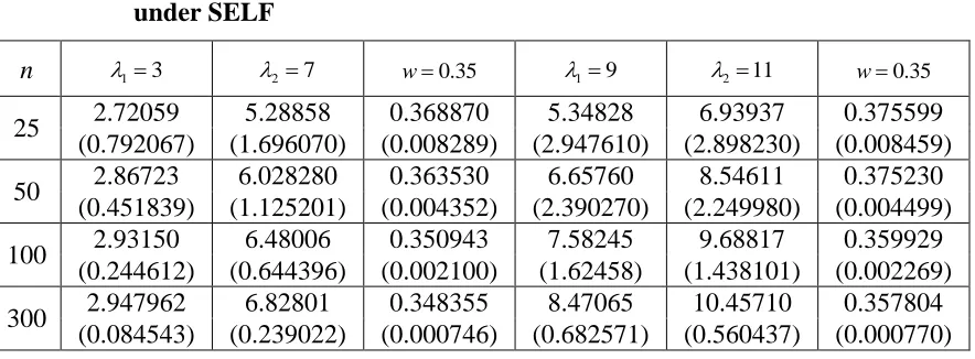
Table 4: Bayes estimates (Exponential) of Burr Type X mixture parameters under SELF
n 13 27 w0.35 19 211 w0.35
25 2.72059 5.28858 0.368870 5.34828 6.93937 0.375599 (0.792067) (1.696070) (0.008289) (2.947610) (2.898230) (0.008459) 50 2.86723 6.028280 0.363530 6.65760 8.54611 0.375230
(0.451839) (1.125201) (0.004352) (2.390270) (2.249980) (0.004499)
100 2.93150 6.48006 0.350943 7.58245 9.68817 0.359929 (0.244612) (0.644396) (0.002100) (1.62458) (1.438101) (0.002269)
300 2.947962 6.82801 0.348355 8.47065 10.45710 0.357804 (0.084543) (0.239022) (0.000746) (0.682571) (0.560437) (0.000770)
Table 5: Bayes Estimates (Uniform) of Burr Type X mixture parameters under PLF
n 13 27 w0.35 19 211 w0.35
25 3.63081 7.81626 0.379789 10.76150 12.36130 0.391052 (0.372643) (0.466748) (0.021960) (1.10449) (0.738157) (0.022816) 50 3.22798 7.30170 0.370674 9.89830 11.58250 0.378963
(0.172190) (0.222966) (0.011806) (0.528004) (0.353685) (0.012049) 100 3.14062 7.12907 0.354127 9.41779 11.31340 0.361765
(0.087854) (0.108429) (0.006196) (0.265448) (0.172076) (0.006358) 300 3.04858 7.06232 0.349588 9.17393 11.096440 0.357110
(0.029090) (0.054014) (0.002135) (0.086752) (0.056676) (0.002203)
Table 6: Bayes Estimates (Jeffreys) of Burr Type X mixture parameters under PLF
n 13 27 w0.35 19 211 w0.35
25 3.97559 8.14414 0.380948 11.6103 12.9970 0.386649 (0.370027) (0.458917) (0.022075) (1.08062) (0.73241) (0.022521)
50 3.46248 7.56759 0.369176 10.2128 11.90650 0.378516 (0.175344) (0.224237) (0.011778) (0.517186) (0.352806) (0.012144) 100 3.25057 7.22929 0.353921 9.73641 11.43030 0.366667
(0.088455) (0.108306) (0.006232) (0.264949) (0.171243) (0.006352) 300 3.06459 7.10131 0.351089 9.23960 11.13260 0.361796
Table 7: Bayes Estimates (Gamma) of Burr Type X mixture parameters under PLF
n 13 27 w0.35 19 211 w0.35
25 4.39203 9.76091 0.378361 12.19460 15.15220 0.386882 (0.352954) (0.437120) (0.022084) (0.979985) (0.678564) (0.022684) 50 3.69332 8.34134 0.368883 10.63280 13.24760 0.380310
(0.172217) (0.217613) (0.011804) (0.495797) (0.345611) (0.012066)
100 3.36767 7.68878 0.354849 9.88059 12.04450 0.364419 (0.087592) (0.107789) (0.006195) (0.256992) (0.168852) (0.006406)
300 3.11248 7.25726 0.349397 9.30716 11.32090 0.356236 (0.028697) (0.036046) (0.002131) (0.085821) (0.056229) (0.002167)
Table 8: Bayes estimates (Exponential) of Burr Type X mixture parameters under PLF
n 13 27 w0.35 19 211 w0.35
25 2.81632 5.44615 0.377792 5.60420 7.22505 0.391388 (0.262129) (0.306887) (0.022090) (0.521610) (0.407127) (0.022505)
50 2.94209 6.07860 0.369035 6.81321 8.63802 0.380553 (0.148991) (0.180117) (0.011772) (0.345029) (0.255956) (0.012140)
100 2.99418 6.48661 0.355187 7.74382 9.65180 0.361397 (0.081478) (0.097179) (0.006215) (0.210726) (0.144598) (0.006318) 300 2.99668 6.83629 0.348832 8.54831 10.55130 0.359814
(0.027978) (0.034746) (0.002128) (0.080078) (0.053628) (0.002168)
Table 9: Bayes Estimates (Uniform) of Burr Type X mixture parameters under WSELF
n 13 27 w0.35 19 211 w0.35
25 3.43773 7.49636 0.344168 10.12221 11.71480 0.350418 (0.381970) (0.468523) (0.023988) (1.124690) (0.732172) (0.024484) 50 3.19497 7.26792 0.351243 9.45622 11.29910 0.356714
(0.177499) (0.227122) (0.012408) (0.525346) (0.353094) (0.012628) 100 3.09010 7.17604 0.343517 9.22026 11.18990 0.355046
(0.088289) (0.110401) (0.006387) (0.263436) (0.172153) (0.006505)
Table 10: Bayes Estimates (Jeffreys) of Burr Type X mixture parameters under WSELF
n 13 27 w0.35 19 211 w0.35
25 2.94121 6.96661 0.343578 8.89329 10.97050 0.351393 (0.367651) (0.46641) (0.024165) (1.111660) (0.731364) (0.024907)
50 2.96825 6.97154 0.349698 8.91495 10.97320 0.363096 (0.174603) (0.224888) (0.012346) (0.524409) (0.349895) (0.012690)
100 2.99877 6.99661 0.345632 9.01686 10.98961 0.351578 (0.088199) (0.109322) (0.006359) (0.263027) (0.171265) (0.006541) 300 3.00289 6.99948 0.347717 8.93985 10.99760 0.353594
(0.028310) (0.036006) (0.002153) (0.085960) (0.056689) (0.002181)
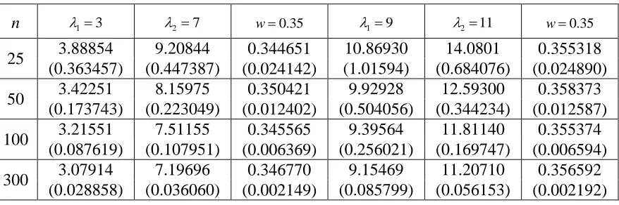
Table 11: Bayes estimates (Gamma) of Burr Type X mixture parameters under WELF
n 13 27 w0.35 19 211 w0.35
25 3.88854 9.20844 0.344651 10.86930 14.0801 0.355318 (0.363457) (0.447387) (0.024142) (1.01594) (0.684076) (0.024890) 50 3.42251 8.15975 0.350421 9.92928 12.59300 0.358373
(0.173743) (0.223049) (0.012402) (0.504056) (0.344234) (0.012587) 100 3.21551 7.51155 0.345565 9.39564 11.81140 0.355374
(0.087619) (0.107951) (0.006369) (0.256021) (0.169747) (0.006594)
300 3.07914 7.19696 0.346770 9.15469 11.20710 0.356592 (0.028858) (0.036060) (0.002149) (0.085799) (0.056153) (0.002192)
Table 12: Bayes estimates (Exponential) of Burr Type X mixture parameters under WELF
n 13 27 w0.35 19 211 w0.35
25 2.42438 5.01342 0.344712 4.83713 6.56521 0.351672 (0.269376) (0.313339) (0.023980) (0.537459) (0.410325) (0.024566)
50 2.74146 5.85477 0.349687 6.31033 8.30897 0.363016 (0.152303) (0.182962) (0.012335) (0.350574) (0.259655) (0.012676) 100 2.85994 6.40238 0.344886 7.36190 9.45204 0.350197
(0.081713) (0.098498) (0.006382) (0.21034) (0.145416) (0.006543) 300 2.95728 6.77115 0.347872 8.41971 0.43219 0.354439
7.1. Graphical Representation of posterior Risks under Different Priors of Component Densities Graphs of Component density 1 Graphs of Component
density 2
Fig. 12. Posterior Risks for
assuming different priors under
WSELF using and
Fig. 9. Posterior Risks for
assuming different priors under WSELF
using
Fig. 7. Posterior Risks for assuming
different priors under SELF using
Fig. 10. Posterior Risks for
assuming different priors under SELF
using and
Fig. 8. Posterior Risks for assuming
different priors under PLF using
Fig. 11. Posterior Risks for
assuming different priors under PLF using
The simulation study has displayed some interesting properties of the Bayes point estimates. The posterior risks of the estimates of the lifetime parameters seem to be quite large (small) for the relatively larger (smaller) values of the parameters. However, in each case the posterior risks of estimates of lifetime parameters are reduced as the sample size increases.
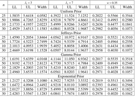
Table 13: The lower limit (LL), the upper limit (UL) and the width of the 95% credible intervals under different priors
n 13 27 w0.35
LL UL Width LL UL Width LL UL Width
Uniform Prior 25 1.5835
7 5.6418 6 4.0582 9 4.3922 7 11.524 1 7.1252 3 0.2022 6 0.5566 7 0.3544 1 50 1.9006
3 4.7265 9 2.8259 6 4.9218 2 9.7879 8 4.8661 6 0.2412 62 0.4993 18 0.2580 6 10 0 2.1733 4 4.1957 1 2.0223 7
5.4999 8.9266 4 3.4267 4 0.2636 07 0.4477 38 0.1841 3 30 0 2.4929 7 3.6513 4 1.1583 7
6.0841 8.0528 5 1.9687 5 0.2982 31 0.4056 25 0.1073 9 Jeffreys Prior
25 1.4590 1 5.2054 3 3.8464 2 4.0562 0 10.972 9
6.9167 0.2010 9
0.5521 4
0.3510 6 50 1.7724
8
4.5223 8
2.7499 4.7424 8 9.5339 5 4.7914 7 0.2405 7 0.4964 2 0.2558 5 10 0 2.1013 5
4.0953 1.9939 5 5.4052 1 8.8058 2 3.4006 1 0.2631 5 0.4434 5 0.1803 0 30 0 2.4669 8 3.6198 7 1.1528 9 6.0507 3 8.0144 4 1.9637 1 0.2958 3 0.4030 3 0.1072 0 Gamma Prior
25 1.6191 6 5.6359 8 4.0168 2 4.1144 6 11.050 7 6.9362 4 0.2017 3 0.5535 5 0.3518 2 50 1.9192
5
4.7315 5
2.8123 4.7730 9 9.5715 2 4.7984 3 0.2409 4 0.4949 4 0.2540 0 10 0 2.1829 2 4.2003 4 2.0174 2 5.4210 2 8.8240 2
3.403 0.2613 1 0.4459 4 0.1846 3 30 0 2.4960 8 3.6535 4 1.1574 6 6.0561 9 8.0203 6 1.9641 7 0.2971 5 0.4028 9 0.1057 3 Exponential Prior
25 1.2127 9 4.3208 6 3.1080 7 4.3922 7 7.9255 2 3.5332 5 0.2019 1 0.5513 4 0.3494 3 50 1.6472
5 4.0964 6 2.4492 1 4.9218 2 8.0110 4 3.0892 2 0.2393 2 0.4961 3 0.2568 0 10 0 2.0127 2 3.8856 3 1.8729 1
5.4999 8.0398 1 2.5399 1 0.2629 2 0.4452 3 0.1823 1 30 0 2.4283 8 3.5567 5 1.1283 7
6.0841 7.7674 6 1.6833 6 0.2978 3 0.4020 7 0.1042 4
Table 13 gives the results for interval estimation. It is interesting to see that all the credible intervals contain the true value of the parameter. The credible intervals tend to be more specific under the assumption of the exponential prior. The width of credible interval is inversely proportional to sample size. The findings of the interval estimation also advocate that in order to estimate 1, 2 and w, the use of exponential prior can be preferred. It should be noted that the credible intervals for the other combination of the parametric values have not been presented as they follow the similar patterns.
9. Real Life Example
This section covers the analysis of real life data set regarding the breaking strengths of 64 single carbon fibers of length 10, presented Lawless (2003). The idea has been to see whether the results and properties of the Bayes estimators, explored by simulation study, are applicable to a real life situation. We have taken n = 64 and T = 3.501 in order to have censoring rate close to 20% (that has been used in simulation study). The results of the analysis have been reported in the following tables. The amounts of posterior risks associated with each estimate have been presented in the parenthesis in the tables.
1 3
27
1 3
27
1 3
Table 14: Bayes estimates and posterior risks under real life data usingw0.35
Loss Function 1 2 w 1 2 w
Uniform Jeffreys
SELF 586.64784 684.96707 0.36710 581.87619 683.80672 0.36561
(5998.50714) (6139.78479) (0.03126) (5963.70792) (6103.83917) (0.03112)
PLF 590.09875 689.01264 0.37445 585.49791 688.33968 0.37322
(6.90183) (8.09115) (0.01469) (7.24344) (9.06591) (0.01520)
WSELF 577.62248 674.96094 0.35092 571.51824 671.49608 0.34893
(9.02535) (10.00612) (0.01618) (10.35795) (12.31064) (0.01668)
Gamma Exponential
SELF 594.25344 709.85097 0.36769 570.01915 666.24748 0.35989
(5954.74938) (6076.50709) (0.03069) (5645.80140) (6006.24078) (0.02945)
PLF 596.46348 713.06151 0.37289 571.94323 668.29623 0.36344
(4.42009) (6.42107) (0.01039) (3.84816) (4.09751) (0.00909)
WSELF 587.48067 700.92605 0.35209 563.57439 660.81255 0.34767
(6.77277) (8.92492) (0.01560) (6.44476) (5.43493) (0.01222)
Table 15: Bayes estimates and posterior risks under real life data using w0.45
Loss Function
1
2 w 1 2 w
Uniform Jeffreys
SELF 578.77102 675.89204 0.44713 574.04339 674.76413 0.44572
(5725.84773) (8807.06835) (0.03831) (5680.47114) (80343.45159) (0.03848)
PLF 582.13541 680.07069 0.45661 577.43224 680.12762 0.45596
(6.72878) (8.35729) (0.01895) (6.67769) (7.72698) (0.02049)
WSELF 571.06410 661.19582 0.42753 566.79832 661.61529 0.42410
(7.70692) (14.69623) (0.01960) (7.24507) (13.14884) (0.02162)
Gamma Exponential
SELF 586.29208 700.42877 0.44837 570.65717 667.87697 0.41940
(5670.51313) (9689.56536) (0.03779) (5280.48484) (7600.81798) (0.03613)
PLF 588.44681 704.01181 0.45426 571.34555 669.45127 0.42444
(4.30948) (7.16607) (0.01178) (1.37675) (3.14860) (0.01007)
WSELF 579.21176 688.99712 0.43218 564.21325 656.67974 0.40908
(7.08031) (11.43165) (0.01619) (6.44392) (11.19723) (0.01332)
parameter of the first component of the mixture. This is due to the reason that the increase in the values of the mixing parameter will add more values for the analysis of the first component of the mixture. Therefore, the findings from the analysis of real life data are in accordance with those of simulation study, suggesting the preference of exponential prior under PLF.
10. Hazard Rate for the Mixture of Burr Type X Distribution
The hazard rate is a useful way of describing the distribution of ‘time to event’ because it has a natural interpretation that relates to the aging of a population. The hazard function is the risk of failure in a small time interval, given survival at the beginning of the time interval. As a function of time, a hazard function may be increasing; meaning as time increases the rate for failure increases, for example, when a patient is untreated for a disease such as cancer or the medication do not work properly; may be decreasing, for example, as a person is recovering from severe trauma like a surgery; or may be constant, meaning the rate of failure is the same regardless of how much time has passed. The constant hazard rate is mostly unrealistic. The hazard rate for the mixture of Burr Type X distribution has been compared under a range of parametric values.
Hazard rate function for mixture of Burr Type X distribution is:
1 2
1 2
1 1
2 2 2 2
1 2
2 2
2 exp 1 exp 1 2 exp 1 exp
1 1 exp 1 1 exp
x x x x x x
H t
x x
(22)
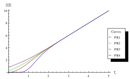
The graphs for the hazard rate of the mixture model, for different parametric values and for the various ranges of the variable, are presented in the following. The abbreviations in the graphs are: HR: hazard rate; PR1: θ1 = 0.50, θ2 = 0.75; PR2: θ1 = 0.75, θ2 = 2.00; θ1 =
1.50, θ2 = 3.00; PR4: θ1 = 2.50, θ2 = 4.00.
Fig. 13: Graph of hazard rates for mixture of model using π = 0.25 and 0 < t < 5
Fig. 15: Graph of hazard rates for mixture of model using π = 0.75 and 0 < t < 5
1 2 3 4 5
t
2 4 6 8 10
HR
P R4 P R3 P R2 P R1 Curves
1 2 3 4 5 t
2 4 6 8 10 HR
Fig. 14: Graph of hazard rates for mixture of model using π = 0.25 and 0 < t < 5
Fig. 16: Graph of hazard rates for mixture of model using π = 0.75 and 0 < t < 5
Fig. 17: Graph of hazard rates for mixture
of model using t = 2 and 0 < π < 1 Fig. 18: Graph of hazard rates for mixture of model using t = 1 and 0 < π < 1
The graphs suggest that the hazard rate for the mixture model tend to decrease for smaller ‘t’ and larger parametric values. However, for t > 3 the choice of parametric values does not have a significant impact on the behavior of the hazard rate. The figures simply suggest that the hazard rate is an increasing function. The increase in the value of the mixing parameter (w) increases the hazard rate. The results are in accordance with the theory; because by increasing the mixing weight there are chances of more failures.
11. Model Comparison Criteria
Bernardo (1979) proposed that under Bayesian inference, the performance of a model is based on the posterior predictive distribution. The criterion used to compare them is based on the use of the logarithmic score as a utility function in a statistical decision. When the uncertainty is contained in the value of a future observation yxn1the logarithmic score log
gk
y x
is used, where gk
y x denotes the posterior predictivedensity under model Mk. Then, the posterior predictive expected utility is given by:
log x x
k k k
U
g y g y dy. The optimal solution to the decision problem of choosing among the competing models M0, M1, .... , Mw is given by the model Mk*, suchthat: *
max
k kU U . Practically, the Ukcan be estimated as: ˆ 1 log
x
m
k k i
U g y
m
.1 2 3 4 5 t
2 4 6 8 10
HR
P R14 P R13 P R12 P R11 Curves
1 2 3 4 5 t
2 4 6 8 10
HR
P R14 P R13 P R12 P R11 Curves
0.2 0.4 0.6 0.8 1.0
3.90 3.95 4.00
HR
P R4 P R3 P R2 P R1 Curves
0.2 0.4 0.6 0.8 1.0
1.0 1.5 2.0 HR
where y1, y2, ... , ym are an independent and identically distributed random sample from
xk
g y . This criterion can be used for selection of a suitable prior for the posterior analysis. The prior for which the posterior predictive distribution produces the maximum amount of posterior predictive expected utilities can be considered to be the best model. The more details can be seen from: Martin and Perez (2009). For numerical illustration, we have generated a random sample of size 30 from mixture of Burr type x distribution with for λ1 = 1.80, λ2 = 2.00 and w = 0.35. The values of the sample are:
Table 16: Simulated sample from mixture of Burr type x distribution for λ1 = 1.80,
λ2 = 2.00 and w = 0.35
0.571361 0.926639 1.102480 1.247594 1.456517 1.689385 0.666807 0.967292 1.137095 1.270262 1.499276 1.715857 0.748350 1.005153 1.162367 1.316861 1.545267 1.848867 0.830025 1.034984 1.190743 1.368140 1.600780 1.940499 0.881668 1.058690 1.215792 1.411192 1.643376 2.127397
Now a sample of size 1000 for the parameters of the posterior distribution under each prior is generated. Based on these samples the estimated values for the posterior predictive expected utilities have been presented in the following table.
Table 17: The posterior predictive expected utilities under different priors
Uniform Jeffreys Gamma Exponential
-1.77146 -1.75013 -1.70721 -1.63065
Now based on these posterior predictive expected utilities it can be assessed that the posterior distribution under exponential prior is the best among all the posterior densities. Hence, the most suitable prior is exponential prior. The findings from the model comparison criteria endorsed the preference of the exponential prior as suggested by the analysis of simulated and real life data sets.
12. Conclusion
References
1. Afify, W. M. (2011). Classical estimation of mixed Rayleigh distribution in type i progressive censored, Journal of Statistical Theory and Applications, 10(4), 619-632.
2. Ahmad, K. E., Fakhry, M. E. and Jaheen, Z. F. (1997). Empirical Bayes estimation of P(Y < X) and characterization of Burr-type X model, Journal of Statistical Planning and Inference, 64, 297-308.
3. Aslam, M. (2003). An application of prior predictive distribution to elicit the prior density, Journal of Statistical Theory and Applications. 2(1), 70-83.
4. Bernardo, J. M. (1979). Expected information as expected utility. Ann. Statist. 7, 686-690.
5. Bolstad, W. M. (2004). Introduction to Bayesian Statistics. John Wiley and Sons, Inc. New York.
6. Burr, I. W. (1942). Cumulative frequency distribution, Annals of Mathematical Statistics, 13, 215-232.
7. Gauss, C. F. (1810). M´ethode des Moindres Carr´es. M´emoire sur la Com-bination des Observations. Transl. J. Bertrand (1955). Mallet-Bachelier, Paris. 8. Demidenko, E. (2004). Mixed Models: Theory and applications. Wiley, New
Jersey.
9. Eberly, L. E. and Casella, G. (2003). Estimating Bayesian credible intervals.
Journal of Statistical Planning and Inference, 112, 115-132.
10. Erisoglu, U., Erisoglu, M. and Erol, H. (2011). A mixture model of two different distributions approach to the analysis of heterogeneous survival data, World Academy of Science, Engineering and Technology, 78, 41-45.
11. Ghosh, S. K. Ebrahimi, N. (2001). Bayesian analysis of the mixing function in a mixture of two exponential distributions. Tech. Rep. 2531, Institute of Statistics
Mimeographs, North Carolina State University, North Carolina State University. 12. Ismail, S. A. and El-Khodary, I. H. (2001). Characterization of mixtures of
exponential family distributions through conditional expectation, Annual Conference on Statistics and Computer Modeling in Human and Social Sciences, 13, 64-73.
13. Jaheen. Z. F. (1996). Empirical Bayes estimation of the reliability and failure rate functions of the Burr type X failure model, Journal of Applied Statistical Sciences, 3, 281-288.
14. Legendre, A. (1805). Nouvelles M´ethodes pour la D´etermination des Orbitesdes Com.etes. Courcier, Paris.
15. McLachlan, G. J. and Peel, D. (2000). Finite Mixture Models, John Wiley and Sons, New York.
16. Martin, J. and Perez, C. J. (2009). Bayesian analysis of a generalized lognormal distribution, Computational Statistics and Data Analysis, 53, 1377-1387.
18. Mendenhall, W. and Hadar, R. J. (1958). Estimation of parameters of mixed exponen-tially distributed failure time distributions from censored life test data.
Biometrika, 45(3-4), 504-520.
19. Nair, M. T. and Abdul, E. S. (2010). Finite mixture of exponential model and its applications to renewal and reliability theory, Journal of Statistical Theory and Practice, 4(3): 367-373.
20. Raqab, M. Z. (1998). Order statistics from the Burr type X model, Computers Mathematics and Applications, 36, 111-120.
21. Saleem M. and Aslam M. (2008). Bayesian analysis of the two component mixture of the Rayleigh distribution assuming the Uniform and the Jeffreys prior from censored data, J. App. Statist. Science, 16(4), 105-113.
22. Saleem, M., Aslam, M. and Economou, P. (2010). On the Bayesian analysis of the mixture of Power function distribution using the complete and the censored sample. J. Applied Statistics, 37(1), 25-40.
23. Saleem, M., Aslam, M. and Economou, P. (2010). On the Bayesian analysis of the mixture of power function distribution using the complete and the censored sample, Journal of Applied Statistics, 37(1), 25-40.
24. Sartawi, H. A. and Abu-Salih, M. S. (1991). Bayes prediction bounds for the Burr type X model, Communications in Statistics - Theory and Methods, 20, 2307-2330.
25. Shi, Y. and Yan, W. (2010). The EB estimation of scale parameter for two parameter exponential distribution under the type-I censoring life test, J. Phys. Sci. 4, 25-30.
26. Sultan, K. S., Ismail, M. A. and Al-Moisheer, A. S., 2007. Mixture of two inverse Weibull distributions: properties and estimation, Computational Statistics & Data Analysis, 51, 5377-5387.