An interactive visualization framework for performance
analysis
Emilio Coppa
Dept. of Computer Science
Sapienza University of Rome
[email protected]
ABSTRACT
Input-sensitive profiling is a recent methodology for analyz-ing how the performance of a routine scales as a function of the workload size. As increasingly more detailed profiles are collected by an input-sensitive profiler, the information conveyed to a user can quickly become overwhelming. In this paper, we present an interactive graphical tool called
aprof-plot for visualizing performance profiles. Exploit-ing curve fittExploit-ing techniques, aprof-plot can estimate the asymptotic complexity of each routine, pointing the atten-tion of the programmer to the most critical routines of an application. A variety of routine-based charts can be auto-matically generated by our tool, allowing the developer to analyze the performance scalability of a routine. Several ex-amples based on real-world applications are discussed, show-ing how to conduct an effective performance investigation usingaprof-plot.
Categories and Subject Descriptors
C.4 [Performance of Systems]: Measurement Techniques; H.5.2 [User Interfaces]: Graphical user interfaces (GUI)
General Terms
Performance, Measurement, Visualization.
1.
INTRODUCTION
Performance optimization is a critical step during software development. Programmers make use of profilers to under-stand the application runtime behavior and to spot perfor-mance bugs. Traditional profilers help developers find out how specific portions of code are responsible for resource consumption, such as memory space and CPU time. Some recent works have made a step further by addressing the problem of designing and implementing performance pro-filers that return, instead of a single number representing the cost of a portion of code, a function that relates the cost to the input size (see, e.g., [4, 9, 21]). These approaches have been inspired by traditional asymptotic analysis of
al-gorithms, and make it possible to analyze – and sometimes predict – the behavior of actual software implementations run on deployed systems and realistic workloads.
This paper is based on the input-sensitive profiling method-ology described in [4]: this approach is able to automatically measure how the performance of individual routines scales as a function of the input size, yielding clues to their growth rate. From one or more runs of a program, an input-sensitive profiler collects several performance measurements related to the runtime behavior of an application and of its rou-tines. These profile data are stored as text-based files and can quickly become very large as increasingly more detailed profiles are collected, making it really hard for a developer to take benefit of this valuable information. To overcome this problem, in this paper we present an interactive graphical viewer for input-sensitive profiles, written in Java and called
aprof-plot. Several routine-based charts can be automati-cally generated by our tool, allowing the developer to ana-lyze the performance scalability of a routine and to obtain useful insights on its workload. Exploiting curve fitting algo-rithms,aprof-plotautomatically estimates the asymptotic complexity of each routine, pointing the attention of the programmer to the most critical routines of an application. Noise reduction techniques and other useful features support the user towards a more effective performance investigation. The tool is available athttp://code.google.com/p/aprof/.
Related work. Performance profiling has been the subject of extensive research since the early 70’s. For many years, analysis of profile data has been performed using command line tools [10], which provides limited user interaction. To-day, the importance of visualization tools for evaluating pro-gram performance has been widely recognized and the ma-jority of integrated development environments (IDEs) offer several interactive visualizers for inspecting the runtime be-havior of an application. VisualVM [19] is a widespread graphical tool, built on top of the NetBeans IDE platform, for profiling the running time and memory usage of Java ap-plications. Several recent works specifically help the user to understand, find, and eventually fix memory-related prob-lems in their programs. AllocRay [17] is an animated in-teractive viewer for memory allocation events which shows the changes of the memory over time using 2D memory map plots. dymem[16] builds a directed acyclic graph depicting group-based object ownership: a compact tree-based rep-resentation of this graph can help a developer to identify common memory problems.
KCachegrind[20] is a well-known data visualization tool for profiles generated by callgrind[20] as well as other open
3HUPLVVLRQWRPDNHGLJLWDORUKDUGFRSLHVRIDOORUSDUWRIWKLVZRUNIRU SHUVRQDORUFODVVURRPXVHLVJUDQWHGZLWKRXWIHHSURYLGHGWKDWFRSLHV DUHQRWPDGHRUGLVWULEXWHGIRUSURILWRUFRPPHUFLDODGYDQWDJHDQGWKDW FRSLHVEHDUWKLVQRWLFHDQGWKHIXOOFLWDWLRQRQWKHILUVWSDJH7RFRS\ RWKHUZLVHWRUHSXEOLVKWRSRVWRQVHUYHUVRUWRUHGLVWULEXWHWROLVWV UHTXLUHVSULRUVSHFLILFSHUPLVVLRQDQGRUDIHH
9$/8(722/6'HFHPEHU%UDWLVODYD6ORYDNLD &RS\ULJKWk,&67
'2,LFVWYDOXHWRROV
source profilers. UsingKCachegrind, besides analyzing how the running time has been spent during the execution of a program, a developer can inspect the call graph and iden-tify performance bugs due to poor cache utilization. To the best of our knowledge, the lack of information about the workload of a routine does not allow these tools to evaluate how the performance of routines scale as a function of the workload size.
Paper organization. The remainder of this paper is orga-nized as follows. In Section 2 we summarize the main ideas behind the input-sensitive profiling methodology. The de-sign and the main features of our graphical tool are covered in Section 3: after discussing the motivation and goals of
aprof-plot, several examples show how our tool can be ef-fectively leveraged by programmers for performance analysis purposes. Section 4 concludes the paper, outlining directions for future work.
2.
PROFILING METHODOLOGY
The main idea behind input-sensitive profiling is to aggre-gate performance measurements for individual routine calls by the size of the input on which each call operates. Dif-ferently from the classical analysis of algorithms based on theoretical cost models, where the input size of a procedure is a parameter known a priori, a key challenge of an auto-mated approach is the ability to automatically infer the size of the data given as input to a function. This can be done using theread memory sizemetric introduced in [4]:
Definition 1. Theread memory size (rms) of the exe-cution of a routinef is the number of distinct memory cells first accessed byf, or by a descendant off in the call tree, with a read operation.
The intuition behind this metric is the following. Consider the first time a memory locationis accessed by a routine activationf: if this first access is a read operation, then
contains an input value forf. Conversely, ifis first writ-ten byf, then later read operations will not contribute to increase therms since the value stored in was produced byf itself.
Notice that the rmsdefinition, which is based on tracing low-level memory accesses made by the program, supports memory dereferencing and pointers in a natural way. How-ever, the rms metric ignores any communication between threads and data received via system calls from the OS ker-nel, failing to accurately characterize the behavior of rou-tines executed in the context of modern concurrent and in-teractive applications. A more recent work [6] has extended therms metric in order to include dynamic input sources such as communication between threads and I/O. For the sake of presentation, in this paper we refer to the original metric, but any consideration can be naturally applied to the latter extension.
Input-sensitive profile. Given a metric for estimating the input size of a routine activation, an input-sensitive profiler collects several performance measures in order to evaluate the routine performance scalability. For each rou-tine f, let Nf = {n1, n2, . . .} be the set of distinct in-put sizes on which f is called during the execution of a program. For each ni ∈ Nf, the profiler collects a tuple ni, ci, maxi, mini, sumi, sqi, where:
benchmark no. routines profile size (MB)
403.gcc 2551 19.2
445.gobmk 1780 36.5
454.calculix 777 9.7
471.omnetpp 1125 2.1
bodytrack 617 3.1
canneal 631 0.8
facesim 776 0.5
ferret 906 16.4
vips 982 47
352.nab 361 3.4
367.imagick 685 0.3
376.kdtree 223 28
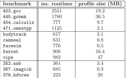
Table 1: Number of routines and profile sizes of sev-eral benchmarks taken from SPEC CPU2006, PAR-SEC 2.1, and SPEC OMP2012.
• ciis the number of times the routine is called on input sizeni;
• maxiandminiare the maximum and minimum costs required by any execution off on input sizeni, re-spectively;
• sumiandsqiare the sum of the costs required by the executions off on input size ni and the sum of the costs’ squares, respectively.
In principle, the term cost may refer to any performance metric, e.g., time, number of executed basic blocks, or cache misses. Since the focus of the input-sensitive profiling method-ology is on modeling scalability rather than on exact running times, the results presented in this article are based on basic block counts, which have several advantages for studying the asymptotic behavior of a program, as explained in [9]. After running an application under an input-sensitive profiler, the programmer gets a text-based profile which contains a dump of all performance tuples collected for any executed routine.
3.
VISUAL MINING OF INPUT-SENSITIVE
PROFILES
As discussed in Section 2, several performance measure-ments are automatically collected by an input-sensitive pro-filer: although these data can be aggregated at runtime ac-cording to several criteria, the resulting profiles may easily become very large due to the high number of routines typ-ically executed by real-world applications. Table 1 shows some profile statistics related to several applications taken from the SPEC CPU2006 suite [11], the Princeton Applica-tion Repository for Shared-Memory Computers (PARSEC 2.1) [2], and the SPEC OMP2012 suite [15]. The profiles have been obtained using the profileraprof-0.2.1[1] while running these applications on their reference workloads. As an example, the GNU Compiler Collection release included in the SPEC suite (403.gcc) has executed more than 2500 distinct routines during our tests, resulting in 19.2 MB of profile data. But even benchmarks with fewer routines lead to huge profiles: for instance, 376.kdtree, with only 223 routines, has generated a 28 MB report.
Input-sensitive profiles are stored as text-based files. From our experience, manual inspection of these files turns out to be largely impractical for a common programmer even with profiles of just few kilobytes. For this reason, we have devel-oped an interactive visualizer written in Java, called
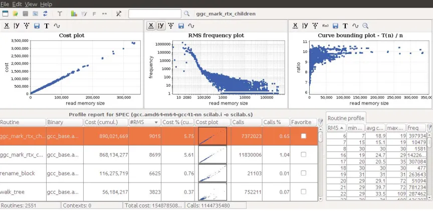
Figure 1: Main window ofaprof-plot: list of profiled routines (bottom left), automatically generated charts (top) and list of performance tuples (bottom right) of a selected routine.
plot. The goal of this graphical tool is twofold. From one side, the user can inspect the scalability of a specific routine by analyzing several routine-based performance charts. On the other side, our tool attempts to focus the attention of the programmer to the most critical routines, possibly pinpoint-ing unexpected performance trends. Before discusspinpoint-ing how
aprof-plotcan support the user towards these two perfor-mance analysis’ directions, we briefly provide an overview of its design. The main interface is shown in Figure 1. Af-ter selecting an input-sensitive profile, a list of routines is presented (bottom left) to the user with several pieces of in-formation for each routine: alongside the routine signature and its executable binary, various cumulative performance metrics summarize the impact on the overall application ex-ecution (e.g., percentage of cost spent inside the routine, number of calls, number of collected performance tuples). Whenever the user selects from this list a specific routine, on the top part of the interface several routine charts are automatically generated. Each plot can be customized by the user through different tools available in the chart ac-tion bar. Finally, the performance tuples collected for the selected routine are listed in the bottom right part of the interface: this allows programmer to carefully inspect the routine profile and to find out details of performance behav-iors graphically represented by the routine charts.
3.1
Routine performance analysis
Performance as a function of workload size. Input-sensitive profiling naturally allows the programmer to inves-tigate how the running time of a routine scales as a function of its workload size. This kind of analysis is actually critical for any software: seemingly benign fragments of code may be fast on some testing workloads, passing unnoticed with traditional profilers, while all of a sudden they can become major performance bottlenecks when deployed on larger
in-puts (see, e.g., examples in [5]). To this aim, aprof-plot
can automatically generate worst-case, average-case, and best-case cost plots. Indeed, given the tuplesni, ci, maxi, mini, sumi, sqi collected for a routine f (see Section 2), the sets of pointsni, maxiandni, minican be used to estimate how the empirical worst-case and best-case costs of a routine grow as a function of the input size. The aver-age behavior is instead given by the setni, avgi, where the average cost per invocation on input sizeniis obtained by computing avgi = sumi/ci. An example of these charts is provided in Figure 2a and is based on routine heap-sort_pairs of SPEC OMP2012 benchmark 352.nab: the best-case, average-case, and worst-case trends appear to be relatively similar and rather smooth.
To get more precise insights on asymptotic performance of a routine, our tool allows the programmer to easily apply a technique known as curve bounding. In particular, the guess ratio rule (see [13] and [14]) estimates the trend of a functionf(n) by considering a guess functionh(n) and an-alyzing the trend of ratiof(n)/h(n): the ratio stabilizes to a non negative constant if f ∈O(h(n)), while it (eventu-ally) increases iff ∈O(h(n)). In our example we divided the worst-case trend of Figure 2a by three different guess functions: n,nlogn, andn2. The three resulting curves are shown in Figure 2b, Figure 2c, and Figure 2d, respectively. The cost of routineheapsort_pairsincreases when divided byn, decreases when divided byn2, and stabilizes to a pos-itive constant when divided bynlogn. This confirms that the trend is nlogn, as expected from any bug-free imple-mentation of the heapsort algorithm. An interactive popup menu, available when displaying the curve bounding plot in
aprof-plot, allows the programmer to easily test several user-defined guess functions.
Workload analysis. A natural question is which are the typical workloads of a routine. Even more interesting is
(a) (b) (c) (d)
Figure 2: Cost plot and curve bounding plots related to routineheapsort_pairsof benchmark352.nab[15].
(a) (b) (c) (d)
Figure 3: (a) Frequency plot of routine heapsort_pairs. Routine std::vector::push back: cost plot (b), fre-quency plot (c), and amortized cost plot (d).
vestigating how the actual workload is impacting the routine performance. Two orthogonal considerations can be made. From one side,aprof-plotcan give insights on the typical workloads on which a routine is called during the execu-tion of a program: as an example, Figure 3a depicts the frequency distribution of the workload sizes observed for routineheapsort_pairs: a peak around thermsvalue 200 provides a rough estimation about the typical size of arrays sorted by this routine in this specific application. In gen-eral, this information might be very useful not only for code optimization, but also for algorithmic improvements, even theoretical, in specific scenarios. For instance, if an applica-tion always needs to sort arrays with less than 16 items, it may be convenient to use a non-optimal sorting algorithm with runtimen2 instead of an asymptotically optimal one with runtimenlogn. A case study of this flavour is dis-cussed in [5].
On the other side, in many scenarios a routine may be gen-erally cheap, but sporadically require a high cost. Consider for instance an operation that appends an item at the end of a resizable array such asstd::vector’spush_back func-tion of the C++ STL. If the array capacity is not exceeded, then the operation takes constant time. Otherwise, the ar-ray must be reallocated, typically requiring an expensive copy of all items from the current array to a new larger one. Expanding the array by a constant multiplicative fac-tor at each reallocation (e.g., doubling the array), the ex-pensive append calls can be guaranteed to be exponentially less frequent than constant append calls [7]. This kind of analysis, which measures the average time of a function over a sequence of invocations, is called amortized analy-sis[18]. The amortized costmetric given in [5] can be be computed in terms of the profiling tuples introduced in Sec-tion 2. Due to lack of space, we omit the definiSec-tion of this metric whose main idea is that the cost of expensive but infrequent calls can be amortized over frequent but cheap calls. Exploiting this intuition, more informative plots can
(a) (b)
Figure 4: Worst-case cost plots of 403.gcc’s routine
cse_basic_block: before (a) and after (b) applying smoothing.
be generated by shaving off expensive peaks, leaving just the points where most of the routine work is performed. For in-stance, Figure 3 reports an example based on C++ STL rou-tinestd::vector::push_back. Even if the cost plot of this routine presents a linear trend (Figure 3b), expensive calls are rather infrequent (Figure 3c). A careful analysis of the routine performance tuples reveals that less than 0.000025% of the routine calls has executed more than 250 basic blocks. The goal of the amortized cost plot is to automatically ex-pose this kind of consideration: as shown by Figure 3d, calls over rms values larger than 80 can be amortized (zeroed points), leaving only inexpensive calls which actually char-acterize most of the routine work.
3.2
Plot customization and noise reduction
aprof-plotsupports different kinds of interaction, allowing the programmer to perform a more effective performance in-vestigation. Several useful features can be triggered by the user in order to customize a routine chart. For instance, the
xandyaxes of a plot can be set to logarithmic scales (see, e.g., Figure 3c). Furthermore, since the interesting behavior
(a) (b)
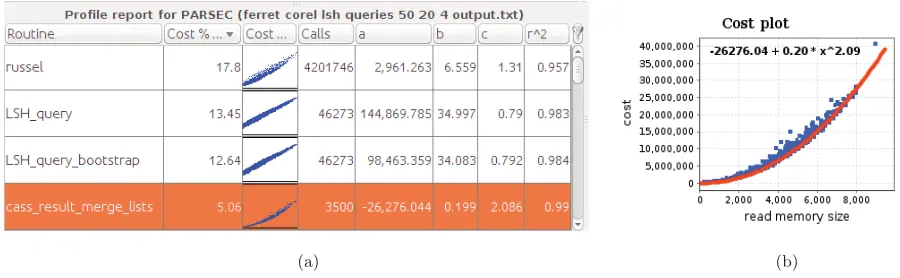
Figure 5: (a) Routine list of PARSEC 2.1 benchmarkferretsorted by percentage of cost, showing preview of cost plot, number of calls, and best-fit parameters. (b) Cost plot of routine cass_result_merge_listswith regression trend obtained by least-squares fitting
of a routine may be confined to a specific area of a chart, the user can zoom in and out from a specific set of points. A common (and more important) issue when analyzing a routine is due to noisy profile data. To this aim, we have implemented two noise reduction techniques: point aggrega-tionandsmoothing. The first approach decreases the num-ber of points, while the second one preserves the cardinality of the original set. Given the set ofNpoints (x, y) of a chart sorted by thexvalues, point aggregation partitions this set in groups ofdpoints and then computes the arithmetic mean within each group. Notice thatdis a positive constant value which can be customized by the user. Smoothing, instead, calculates the centered moving average [12]:
∀k, w
2 ≤k≤N−
w
2 : yk = 1
w k+w/2
i=k−w/2
yi
where w is the user-customizable size of the moving win-dow. Figure 4b provides an example based on the routine
cse_basic_block of the SPEC benchmark 403.gcc: the original noisy trend (Figure 4a) has been smoothed applying a moving windoww= 256.
Finally, we implemented inaprof-plota source code brows-ing feature that allows the programmer to analyze the code while she is still looking at the routine charts. After choosing the source directory of a C/C++ application, aprof-plot
can automatically open the appropriate source code file and show the relevant piece of code inside a text-editor widget. This makes it easier for programmers to find out why a cer-tain piece of code exhibits some performance behaviors.
3.3
Spotting critical routines
In Section 3.1, we have discussed howaprof-plotcan enable a deep analysis of relevant aspects of a routine’s behavior. However, since real-world applications may be composed by thousands of routines, this kind of analysis could easily be-come overwhelming for a developer. For this reason, aprof-plotattempts at pointing the attention of the programmer to the most critical routines of an application. In particular, it helps developers prioritize their analysis by highlighting routines which are likely to contain performance issues. By sorting routines based on the percentage of cost, a devel-oper can immediately understand how the running time has
been spent during the execution of the program. Several filtering strategies can help to refine this list: uninteresting routines, such as library functions, can be filtered out based on the executable binary, while insignificant routines can be hidden using different metric thresholds (e.g., by filtering routines with small cost percentage or with a small number of performance tuples). Exploiting these tools, the number of routines which needs to be analyzed by a developer can be significantly reduced. However, since the ultimate goal of input-sensitive profiling is to detect the routines with high asymptotic cost, we have implemented in aprof-plot an automatic approach for estimating the asymptotic complex-ity of a routine. Using regression analysis techniques [3], our tool constructs for each routine a mathematical func-tion that has the best fit to its data points. In particular, we choose as a cost model the function b·nc+a, which generalizes both the power law and the linear models (when
a= 0 andc= 1, respectively).
After estimating the fitting coefficients for any program rou-tine,aprof-plotcan sort routines based on their asymptotic complexity (i.e., theccoefficient), allowing the developer to possibly detect unexpected performance trends. Since this kind of analysis crucially depends on the quality of the fit-ting results, aprof-plot allows the user to filter routines which have low fitting quality (e.g.,R2≤0.92) or unrealis-tic coefficient values (e.g.,b <0.001). The validity of this approach has been empirically assessed in [5].
Figure 5a provides an excerpt taken from the routine list of the PARSEC benchmarkferret. The original 906 routines have been filtered according to the following criteria: more than 10 performance tuples (|N|>10), high fitting quality (R2 >0.92), and reasonable bcoefficient value (b >0.01). After filtering, 75 routines remain and are sorted based on the percentage of executed basic blocks (i.e., their cost): among the top four routines (shown by Figure 5a), an inter-esting example is provided by cass_result_merge_lists. This routine has been called 3500 times, requiring 5.06% of the total program cost, and aprof-plot has been able to automatically estimate a quadratic asymptotic complex-ity (c = 2.086). As discussed in [5], apart from specific algorithmically-critical routines usually well known to the programmer, most benign routines appear to have a sub-quadratic trend and many common programming mistakes tend to introduce quadratic inefficiencies, e.g., by invoking a
subroutine in a loop under the incorrect assumption that it takes constant time. Since the fitting quality is rather high (R2 = 0.99), routine cass_result_merge_listsis a good candidate for further performance investigation. The worst-case cost plot is given in Figure 5b: the regression curve accurately predicts the actual cost trend. By inspecting the source of this routine, we were able to conclude that its al-gorithm is indeed Θ(n2) due to a doubly-nested loop used for merging two input lists. Although this quadratic trend is not given by any trivial programming mistake, we believe that some algorithmic optimizations could be implemented to improve the running time of this routine.
As shown by this example, the filtering and ranking strate-gies implemented by aprof-plotcan significantly support the developer towards performance investigation of the most critical routines, possibly revealing unexpected performance issues.
4.
CONCLUSIONS
In this paper we have presented an interactive visualization framework for performance analysis of input-sensitive pro-files. The key benefit ofaprof-plotis to allow the program-mer to investigate how the running time of a routine scales as a function of the workload size. Exploiting techniques such as curve fitting and bounding, our tool can focus the attention of the programmer to the most critical routines of an application, possibly pinpointing unexpected scalability problems. Useful insights on the typical workload sizes can help developers optimize their programs.
As a future direction, it would be interesting to improve the support inaprof-plot for input-sensitive profiles with calling-contexts annotations [8]. This further level of perfor-mance characterization can help developers analyze routines with context-dependent performance trends.
Another interesting improvement would be to implement ad-hoc fitting algorithms, specifically tailored to curves related to execution costs. In particular, we notice that a routine may exhibit rather different performance trends based on several runtime conditions and workload features. Since a classical curve fitting algorithm is unable to detect multi-ple trends, aplot-plotfails to automatically estimate the asymptotic complexity of the routine, forcing the user to-wards manual performance analysis.
Acknowledgements
We would like to thank Camil Demetrescu and Irene Finoc-chi for their valuable feedback during the development of
aprof-plot and for many useful discussions. We are also indebted to Bruno Aleandri for developing an earlier ver-sion ofaprof-plot.
5.
REFERENCES
[1] aprof: an input-sensitive profiler.
https://code.google.com/p/aprof/.
[2] C. Bienia, S. Kumar, J. P. Singh, and K. Li. The PARSEC benchmark suite: characterization and architectural implications. InPACT, pages 72–81, 2008.
[3] J. M. Chambers, W. S. Cleveland, B. Kleiner, and P. A. Tukey.Graphical Methods for Data Analysis. Chapman and Hall, New York, 1983.
[4] E. Coppa, C. Demetrescu, and I. Finocchi. Input-sensitive profiling. InProc. of the 33rd ACM SIGPLAN Conf. on Programming Language Design and Implementation (PLDI), pages 89–98, 2012. [5] E. Coppa, C. Demetrescu, and I. Finocchi.
Input-sensitive profiling.IEEE Transactions on Software Engineering, 2014. To appear. [6] E. Coppa, C. Demetrescu, I. Finocchi, and
R. Marotta. Estimating the empirical cost function of routines with dynamic workloads. In12th Annual IEEE/ACM Int. Symposium on Code Generation and Optimization (CGO), pages 230–239, 2014.
[7] T. H. Cormen, C. E. Leiserson, R. L. Rivest, and C. Stein.Introduction to Algorithms. MIT Press and McGraw-Hill, 2009.
[8] D. C. D’Elia, C. Demetrescu, and I. Finocchi. Mining hot calling contexts in small space. InPLDI, pages 516–527, 2011.
[9] S. Goldsmith, A. Aiken, and D. S. Wilkerson. Measuring empirical computational complexity. In
ESEC/SIGSOFT FSE, pages 395–404, 2007. [10] S. L. Graham, P. B. Kessler, and M. K. McKusick.
gprof: a call graph execution profiler (with retrospective). In K. S. McKinley, editor,Best of PLDI, pages 49–57. ACM, 1982.
[11] J. L. Henning. SPEC CPU2006 benchmark descriptions.SIGARCH Comput. Archit. News, 34:1–17, 2006.
[12] MATLAB documentation: moving average filter.
http://www.mathworks.com/help/econ/ filtering.html.
[13] C. C. McGeoch, D. Precup, and P. R. Cohen. How to Find Big-Oh in Your Data Set (and How Not to). In
IDA, pages 41–52, 1997.
[14] C. C. McGeoch, P. Sanders, R. Fleischer, P. R. Cohen, and D. Precup. Using finite experiments to study asymptotic performance. InExperimental Algorithmics, LNCS 2547, pages 93–126, 2002. [15] M. S. M¨uller andet al.SPEC OMP2012 – an
application benchmark suite for parallel systems using OpenMP. InProc. 8th Int. Conf. on OpenMP in a Heterogeneous World, pages 223–236, 2012.
[16] S. P. Reiss. Visualizing the Java heap. InProc. of the 32Nd ACM/IEEE Int. Conf. on Software Engineering, ICSE ’10, pages 251–254, 2010.
[17] G. G. Robertson, T. Chilimbi, and B. Lee. Allocray: Memory allocation visualization for unmanaged languages. InSOFTVIS, pages 43–52, 2010. [18] R. E. Tarjan. Amortized computational complexity.
SIAM Journal on Algebraic and Discrete Methods, 6(2):306–318, 1985.
[19] Visual VM: All-in-One Java Troubleshooting tool.
http://visualvm.java.net/.
[20] J. Weidendorfer, M. Kowarschik, and C. Trinitis. A tool suite for simulation based analysis of memory access behavior. InInt. Conf. on Computational Science, volume 3038 ofLNCS, pages 440–447, 2004. [21] D. Zaparanuks and M. Hauswirth. Algorithmic
profiling. InProc. of the 33rd ACM SIGPLAN Conf. on Programming Language Design and
Implementation (PLDI), pages 67–76, 2012.
![Figure 2: Cost plot and curve bounding plots related to routine heapsort_pairs of benchmark 352.nab [15].](https://thumb-us.123doks.com/thumbv2/123dok_us/8419810.1693734/4.612.322.547.313.408/figure-cost-curve-bounding-related-routine-heapsort-benchmark.webp)