www.ijaera.org 2016, IJA-ERA - All Rights Reserved 270
Extended Great Deluge Metaheuristic based
Approach for the Integrated Dynamic Berth
Allocation and Mobile Crane Assignment
Problem
El Asli Neila1*, Dao Thien-My1, Bouchriha Hanen2
1Mechanical and Industrial Engineering, Ecole de Technologie Supérieure (ETS), Montreal, Canada 2Industrial Engineering, National Engineering School of Tunis (ENIT),Tunis, Tunisia
Abstract: In order for terminals to accommodate the growth in International container transport, they must make significant changes to maintain their position with increasing demand. One important manner in which existing terminal capacity could be increased would be through more efficiency. In this paper, we consider terminal efficiency from the perspective of simultaneously improving both berth and quay crane scheduling. The approach is applied to a discrete and dynamic berth allocation and crane assignment problem for both mono-objective and multi-objective variants. The problem is solved through a neighborhood meta-heuristic called the Extended Great Deluge (EGD). The results obtained with this meta-heuristic have shown better results than a Genetic Algorithm proposed in other works. A Simulated Annealing algorithm (SA) is also implemented to serve as basis of comparison for new instances results. Both algorithms (EGD and SA) for mono-objective variant have been applied to different size instances based on real world and generated data. Two new EGD-based multi-objective approaches have been proposed. Computational results are presented and discussed.
Keywords: Berth Allocation Problem; Container Terminal; Crane Assignment Problem, Extended
Great Deluge; Meta-Heuristic; Multi-Objective Optimization; Simulated Annealing
I. INTRODUCTION
This Container terminals are the areas where containers are transported from one point to another one using different handling equipments. Such terminals are continually growing in importance as maritime transport faces the challenge of using new technologies to build larger and larger ships. Moreover, transport frequency is only rising as commercial exchanges are developed to meet economic growth. To be able to compete within this environment, container terminals must be managed efficiently. To that end, managers must concentrate on the Berth, which is the most critical resource for determining container terminal capacity. An alternative approach to increasing Berth capacity involves improving its productivity through its efficient use [1]. One of the components of such efficient utilization is a focus on quay cranes, which are the main equipment used to move containers at terminals.
www.ijaera.org 2016, IJA-ERA - All Rights Reserved 271 Recently, other studies have examined the two problems simultaneously, because they are actually encountered and do interact in a container terminal. In fact, the goal of a Crane Assignment Problem (CAP) is to determine the total time of docking at the quay (including the time of service: loading/unloading and waiting time), which represents an input of the Berth allocation problem (BAP). Modeling both problems simultaneously thus approximates the reality of the harbor; consequently, resolving the joint problem would allow immediate application by a harbor manager. The combination of both the BAP and the CAP leads to an interesting problem called the BACAP (Berth Allocation and Crane Assignment Problem); this combination attracts more and more the interest of researchers in the field. The concept was pioneered by Park and Kim [1], who modeled the problem in its static-continuous variant as an Integer Programming model, and adopted a two-phase resolution approach. The term static refers to static handling time problem, where vessel handling times are considered as input parameters whereas and by analogy the term dynamic refers to dynamic handling time where handling times are considered as decision variables since the number of cranes are also decision variables. The discrete versus continuous problems refer to the topology of the quay where in the discrete variant the quay is viewed as a finite set of berths whereas in the continuous ones, vessels can berth anywhere along the quay.
Meisel and Bierwirth in [2] were interested in the continuous-dynamic variant, and they classified the problem as a Resource Constrained Project Scheduling Problem (RCPSP). A discrete dynamic variant was studied by Liang in a mono-objective [3] and multi-objective form [4]. They modeled the problem in a very simple and comprehensive way and adopted the genetic algorithm for the resolution. Imai et al. in [5] focus on the discrete-dynamic version. Their modeling objective was the minimization of the total time of service, including the constraints of the CAP. The resolution was based on the genetic algorithm, which is considered among the dominant algorithms proposed in the literature to solve such problems. This finding is presented by Bierwith and Meisel [6] in their recent follow survey of berth allocation and quay crane scheduling problems.
Meisel and Bierwirth [7] used the model suggested by the pioneers [1], and proposed a one-phase resolution based on the construction of a feasible solution, which was then further improved by meta-heuristics. Bierwirth and Meisel in [6] and [8] were interested in the review of the literature on the integration of BAP and CAP problems. They listed the models formulated for the BACAP (Berth allocation and Crane Assignment Problem) and those used in resolutions have been proposed over the last ten years. They concluded that there is a growing interest in such problems relating to in container terminal management, and thus they encourage future researchers to find new models which should be more realistic and new effective resolution methods. According to the same authors in [6], it‘s not surprising that heuristics and meta-heuristics approaches dominate the resolution approaches in the literature since the berth allocation problem is known to be NP hard. Among the heuristic approaches genetic algorithm take the largest part. We can find other meta-heuristics like Tabu Search [9], Ant colony [10], and simulated annealing [11]. Another set of studies have adopted specific heuristics like local search [12] and greedy rules [13]. According to Bierwirth and Miesel [6], specific local search algorithms, meta-heuristics, especially mathematically driven heuristics and exact methods have been under represented so far. They have also conclude that GA are used for their ease of implementation, however, these approaches are often rough and limited in regard to solution quality. This is the reason for our choice for local search metaheuristics. In fact, for this specific model, this work tries to propose a specific heuristic and neighborhood search method to improve the solution quality.
www.ijaera.org 2016, IJA-ERA - All Rights Reserved 272 Neighborhood search heuristics to obtain near optimal solutions in a practical use and within a relatively short amount of time. A comparison between the results of the two algorithms shows the efficiency of the EGD.
In the next section, the mathematical models for both mono-objective and multi-objective variants are presented and detailed. In section 3 the methodology adopted to solve the mono-objective variant by the EGD and SA is explained, which is the first contribution in this study. In section four, and because the EGD present the best results for the mono-objective variant, two new multi-objective algorithms based on the Extended Great Deluge meta-heuristic and the dominance principle are proposed and this represents a second contribution in this paper.
II. BACAP PRESENTATION
A. Liang's problem [3, 4]
Among several BACAP problems encounter in the literature, we consider the one presented [3, 4] in its discrete-dynamic variant. The problem is chosen for its simplicity of comprehension and because it is inspired from a real container terminal in China. The first objective [3], presented as the total time minimization makes the model very generalizable, and capable of being applied to most container terminal situations.
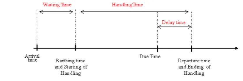
The authors approached the problem to determine the exact position and the berthing time of each ship arriving at the quay of a port, as well as the exact number of Quay Cranes assigned to each of them in order to minimize the total time of berthing to the quay. This includes:
The time of loading/unloading,
Waiting time between arrival time and starting service
The time associated with the difference between the end of the service and the time of departure of the container ship estimated and programmed by the managers (Fig. 1).
Figure 1: Berth Operation Timeline
Their second objective in [4] is the minimization of the workload standard deviation of cranes, considered an indicator of the efficiency of the terminal. This objective guarantees a balanced crane assignment between berths.
www.ijaera.org 2016, IJA-ERA - All Rights Reserved 273 Each container ship has a maximum number of cranes to be assigned.
The time service of a container ship is directly dependent on the number of cranes assigned
It is assumed that the time of arrival of the ship container to the port is known in advance, but the ship cannot berth before the expected arrival time.
Loading/unloading operations must be carried out without interruption.
Each zone of accosting must be able to accommodate a maximum of one container ship.
The crane transfer time is ignored.
B. Problem Formulation
The mathematical model for the discrete-dynamic berth allocation and assignment problem proposed in [3, 4] is presented below.
We define the following indices, parameters and decision variables to formulate it :
Indices:
i (= 1, 2…n) ϵ V set of ships
j (= 1, 2…m) ϵ B set of berths
k (= 1, 2…n) ϵ O set of service orders
Parameters:
n : number of ships
m : number of berths
ν : working speed of the cranes
b : the maximum number of quay cranes that can be assigned to each ship
H : the total number of cranes available in the port
ai : arrival time for ship i
ci : number of containers required for loading/unloading of ship i
di : departure time for ship i.
Decision variables:
si : starting time for serving the ship i
www.ijaera.org 2016, IJA-ERA - All Rights Reserved 274 A: the average working time of cranes
Uj are the working times of cranes on berth j.
1 if if the ship i is served as the kth ship at the berth j
xijk
0 otherwise
n i m j nk j i ijk
i i n i m j n k ijk i i ijk n i m j n k j i x d h c s x a s x h c Min
1 1 1
*) * (*
1 1 1
(**) (*)
1 1 1
1 ) . ( ) ( . Z (1)
H 1M in Z2 h Uj A 2 m j j
(2) Subjection to ) .... 2 , 1 ( 1 1 1 n i x m j n kijk
(3)
n) (1,2,... k , ) .... 2 , 1 ( 1 1
m j x n i ijk (4) j bhj (5)
i a
si i (6)
ljk l k ij j i
i x s x
h c
s
, 1 .
, i,k,l(1,2,...n), j(1,2....m) (7)
H 1
m j j h (8) i integer j h (9) , . . U1 1 1
j x j
h c ijk n i n k j i m j
(10)
.U h H 1 A m 1 j j j
(11)www.ijaera.org 2016, IJA-ERA - All Rights Reserved 275 (**) and finally the delay time for every ship (***). The objective (2) is minimizing the workload standard deviation of cranes. Constraint (3) assures that every ship must be served at some berth in any order of service. Constraint (4) indicates that a ship must be served ones and exactly one at any berth. Constraint (5) restricts the maximum number of cranes used on each ship. Constraint (6) ensures that ships are served after their arrival. Constraint (7) guarantees that the handling of a ship starts after the completion of handling of its immediate predecessor at the same berth. Constraint (8) indicates that each crane on berth could be assigned. Constraint (9) enforces the number of cranes allocated to a ship to be an integer. Constraints (10) and (11) define working time and average working time between berths.
After having presented the problem formulation above, in the following section, the emphasis will be on the first objective. A new effective approach based on a local search will be presented, experienced and tested. Thereafter, in the section 5, the problem in its multi-objective form will be considered.
III. RESOLUTIONMETHODOLOGYFORTHEMONO-OBJECTIFPROBLEM
As presented above, the Liang's model represents hard constraints that make the resolution by meta-heuristics meeting much of non-feasible solutions that the algorithm must circumvent. For this reason, a population method such as the genetic algorithm is not fully appropriate for such problems.
In this paper, and to mitigate the obstacle above mentioned, we propose to solve Liang’s BACAP with a new heuristic method based on neighborhood search. The Extended Great Deluge meta-heuristic is then applied. Prior to that, a meta-heuristic is constructed to find the first feasible solution, which is gradually improved with the exploration of the neighborhood by the metaheuristic algorithm. This is what differentiates the approach suggested in this research from the resolution suggested in [3], which sets on a random initial solution. Moreover, the construction of the initial feasible solution aims to increase the rate of acceptance of the meta-heuristic, which results in increasing the efficiency and speed of the resolution.
Besides the application of another type of algorithm to solve the problem, our approach allows to integrate the priority aspect as a decision strategy for the user. In fact, unlike Liang’s approach, we add constraints relatively to the priority service in case of arbitrage between two arrivals. The approach suggested in this paper is to adopt the First Come First Serve (FCFS) rule. In case of arbitrage between two arrivals or more, the user can choose between the following rules: the “Most charged First” rule, “Less Charged First” rule and finally “Earliest Delivery Date” rule. Such a context could arise in order to satisfy some customers. The harbor manager could then have different scheduling scenarios and decide which strategy to adopt.
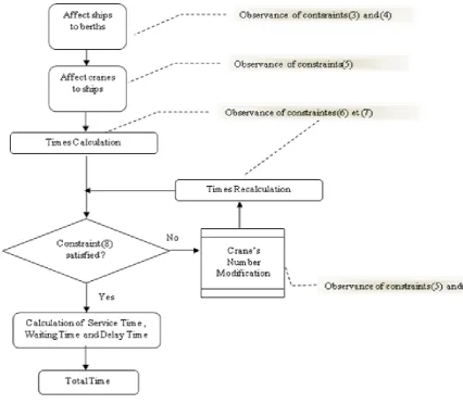
A. Construction of Initial Solution Heuristic
Before the application of the meta-heuristic, a heuristic is constructed to find the first feasible solution, which is gradually improved with the exploration of the neighborhood by the meta-heuristic algorithm. This is what differentiates the approach suggested in this research from the resolution suggested in [3], which sets on a random initial solution. In general, it is expected that the better the initial solution, the better the final solution.
www.ijaera.org 2016, IJA-ERA - All Rights Reserved 276 test is launched to make sure that at any moment the total number of cranes used does not exceed the total number available. If the test fails, a modification to some crane assignments is allowed.
A recalculation of the starting times, the waiting times, the delay and the total time is then performed.
The result is the initial solution that will be gradually improved by the meta-heuristic. The heuristic is repeated until obtaining an upper bound Total Service specified by the user. Fig. 2 presents the several steps of the initial solution construction heuristic.
Figure 2. Initial Solution Construction Heuristic
IV. EXTENDEDGREATDELUGEMETA-HEURISTICVSSIMULATEDANNEALING
www.ijaera.org 2016, IJA-ERA - All Rights Reserved 277 has to be adjusted. According to [14], founder of the method, this parameter can be interpreted as a function of expected search time and expected solution quality, which are relatively easy to specify.
For the application of this algorithm to our problem, we needed:
The initial solution S found by the constructed heuristic.
The definition of the neighborhood N(S) of this solution.
The neighborhood was created while making minor modifications to the initial solution S, such as to the permutation between two container ships taken randomly.
The permutation was done for both the berth and the cranes assignment. Following the modifications, the algorithm applied tests on the neighborhood solution to check if all the constraints have been fulfilled.
Improvement regarding initial solution is carried out through implementation of the EGD algorithm presented in Table 1. As mentioned above, it uses a boundary B, which is initially set equal to the initial solution, and is reduced gradually through the improvement process.
Besides the EGD implementation, a simulated annealing (SA) algorithm is used too in this paper to compare the results for new instances. The same heuristic for the initial solution construction is considered before its improvement by the simulated annealing algorithm. In Table 2, the famous traditional SA is described.
Table I. Extended Great Deluge algorithm
The simulated annealing is also a neighborhood search probabilistic meta-heuristic which emulates the physical annealing process in metallurgy. In the SA, The acceptance criterion with the probability p (T,s,s*) is employed between successive iterations.
Here, the candidate solutions with less objective function values than the current one are accepted with the probability p (T,s,s*) ,where T is a parameter called the «temperature» which is usually gradually reduced during the search. The reduction scheme that is employed is known as the «cooling schedule». Table 1: Extended Great Deluge Algorithm
We can conclude, then, that the SA is using more than one control parameter, which makes it less convenient to use by comparing it to the EGD. According to [14], «…a greater number of poor
Set the initial solution S
Calculate initial cost function f(s)
Initial ceiling B=f(s)
Specify input parameter ∆B=?
While not stopping condition do Define neighbourhood N(s)
Randomly select the candidate solution S* Є N(s)
If (f(s*) ≤ f(s)) or (f(s*) ≤ B) Then Accept S*
Lower the ceiling B = B - ∆B
www.ijaera.org 2016, IJA-ERA - All Rights Reserved 278 quality solutions are generated through the use of inappropriate parameter values for the SA… Although both methods can have approximately the same values of the cost function for the best results, Simulated Annealing can reach it only with properly defined parameters, while Great Deluge does it always. ». For more details about the SA algorithm, we refer the reader to [11].
Table II. Simulated Annealing algorithm
V. PRIORITYRULESINCLUDEDINTHEMODEL
In this paper, in comparison with Liang et al.’s approach [3], we wish to include more priority rules.
1. Like Liang’s approach: First Come First Served (FCFS) rule.
This constraint is modeled as follows:
2. FCFS rule like (1) and when 2 ships assigned to the same berth have the same time arrival, we prioritize the most charged one.
(12i)
3. FCFS rule like (1) and when 2 shi ps assigned to the same berth have the same time arrival, we prioritize the less charged one.
4. FCFS rule like (1) and when 2 ships assigned to the same berth have the same time arrival, we use the Earliest Delivery Date (EDD) rule .
Set the initial solution S
Set the initial temperature T? Calculate initial cost function f(s) Specify input parameter ∆T=? While not stopping condition do Define neighborhood N(s)
Randomly select the candidate solution S* Є N(s) Randomly select r ϵ [0, 1]
p(T,s,s*) = exp ( - ( f ( s *)-f ( s ) ) / T ) If r ≤ p(T,s,s*)
Then Accept S*
www.ijaera.org 2016, IJA-ERA - All Rights Reserved 279
VI. EXPERIMENTSANDCOMPUTATIONALRESULTS
In the following, several experiments have been performed. To begin, solution in [3] found by the genetic algorithm is compared to our EGD result. Then, and to try to generalize the EGD performance, we have taken data from benchmark in [1], which provide different size problems ranging from small to large instances. Another work [15], presenting useful inputs to our BACAP has been taken as another source data.
A. Comparison with Liang’s approach
The aim of this section is to compare the results obtained with our approach with those obtained in [3], where the authors applied their method to solve a real case, coming from one of Shanghai container terminal companies in China. In that case, there were 4 berths and 7 quay cranes. The working speed of quay crane is common to all the cranes and was set to 40TEU/h. The data concerning the arrival time, the due time and the capacities of the ships are shown in the Table 3(in the appendices).They represent a-one day real case data from one of Shanghai container terminal companies in China, for 11 ships/day.
After finding a feasible solution by the initial solution construction heuristic, we dealt with the EGD parameters tuning to ensure good quality of the final solution. The highlight of the EGD is that it has only two parameters to adjust, which are the number of iterations Niterations and the step ∆B. For the latter, Burke in [14] suggests, the formula (13) to calculate, if some information about the range of possible result is available.
(13)
Where f(s’) is the cost function of a desired result.
Table III. Liang’s Ship informations
Ship Name Arrival Time Due Time Total number of container loading/unloading (TEU)
1 MSG 09:00 20:00 428
2 NTD 09:00 21:00 455
3 CG 00:30 13:00 259
4 NT 21:00 23:50 172
5 LZ 00:30 23:50 684
6 XY 08:30 21:00 356
7 LZI 07:00 20:30 435
8 GC 11:30 23:50 350
9 LP 21:30 23:50 150
10 LYQ 22:00 23:50 150
www.ijaera.org 2016, IJA-ERA - All Rights Reserved 280 In our case, Liang and al in [3] have tried to find a near-optimal solution to the problem and hence f(s’) is fixed.
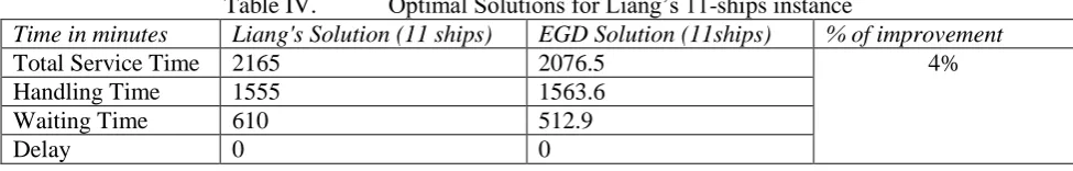
For the parameters’ tuning we adopt (13) for different Niterations (1000, 2000, 5000 10 000, 20 000, 30 000, 50 000 and 100 000). For each combination, the EGD is applied several times. The best results for the 11 ships instance, presented in Table 4, are provided with the parameters Niterations = 50 000 and ∆B=5.10-4. Our best solution is 90 minutes less than Liang’s one, which represent 4% of improvement. We also found several solutions which are lower than the near-optimal one (2165 minutes) found in [3] which could suggest that the EGD outperforms the Genetic algorithm to find a better solution for this specific problem and for this size of instances.
Table IV. Optimal Solutions for Liang’s 11-ships instance
Time in minutes Liang's Solution (11 ships) EGD Solution (11ships) % of improvement
Total Service Time 2165 2076.5 4%
Handling Time 1555 1563.6
Waiting Time 610 512.9
Delay 0 0
The EGD solution provide as well as the GA solution no delay time, a handling time slightly higher than the AG, but a waiting time and consequently a total service time significantly lower than the genetic algorithm. This solution is more interesting for the customer finding the service more satisfying.
B. Comparaison with [1] Benchmark & [15] data set.
Unfortunately, in [3], the authors did not provide other instances with different sizes. This is the reason why, to generalize our approach, and in addition to the real case instance with 11 ships, we use data from a benchmark proposed in [1] (for another kind of BACAP) from where we used 23 real case problems between 13 and 40 ships during the planning horizon. Of course, the benchmark was further expanded in terms of their model’s data, this is why, and we simply used some data that are useful to us. We have also been forced to convert service time assumed as input in their model into a number of containers (by a simple multiplication by the cranes ‘speed).
To verify the performance of our EGD, and because we do not have near–optimal solutions by others meta-heuristics to compare the results, we solved these real case problems by an implemented a traditional simulated annealing (SA) algorithm which uses the same initial solution construction heuristic. We compare the results of the two meta-heuristics to highlight the advantage of using the EGD.
In the Table 5 (see appendices), an example of Park& Kim’s data is presented. We have here 15 ships and the plan horizon is one week. (Greater than the 24 hours plan horizon of [3].We also noticed that the loading capacity of ships is widely greater than which in [3]. We have set the number of berths to 4 [1], the authors considered the continuous variant of BACAP whereas Liang ‘s and al. in [3] studied a discrete variant) , and the number of cranes to 7 .
Another interesting instance is that of [15], which is also used and solved by both EGD and SA. Table 6 shows the input data extracted from [15] data set. There are 21 ships, 4 berths, 7 cranes and one week horizon plan.
www.ijaera.org 2016, IJA-ERA - All Rights Reserved 281 Table V. Ships instance Information
URSAVAS Ship name Arrival Time (hour)
Due Time (hour)
Total number of container loading/unloading (TEU)
1 MSC1 6.25 31 330
2 NPT 17 42 873
3 MRS1 24.5 49 358
4 HMS1 24 49 517
5 WW1 25.833 50 122
6 KPE1 26.416 51 621
7 VDB1 32.833 57 210
8 ORK1 41.5 66 1336
9 WND1 42.5 67 380
10 LYQ1 45,833 70 349
11 MAR1 50 74 885
12 MSC2 51,25 76 214
13 MRS2 64,5 89 668
14 HMS2 72,66 97 236
15 WW2 90,75 115 1310
16 KPE2 101,5 126 573
17 VDB2 106,33 131 615
18 ORK2 111,58 136 401
19 WND2 129,75 155 608
20 LYQ2 130,25 156 130
21 MAR2 151,25 176 1830
As presented previously, 22 real cases and 6 generated cases were taken from [1], distributed as follow: for the real cases, 4 problems with 13 ships each , 4 x 14 ships , 2 x 15 ships , 7 x 16 ships and 5 x 17 ships. For the generated ones, 2 x20 ships, 2x30 ships and 2x 40 ships.
We classify these instances according to their sizes in small (13-15ships), medium (16-17ships) and large (20-40 ships) classes. In the following tables (7, 8 and 9) we present the solutions found for the different classes of real case problems and generated ones with both EGD and SA.
For each size instances, and in order to verify the homogeneity of data, we have looked more closely at the ship loading average, the average stay and the average inter- arrival of ships. For the different size instances, we have noticed a consistency between the same size data, and this is due to the fact that they are of the same terminal. The problem size is presented in the first colons as follows: number of ships instance number.
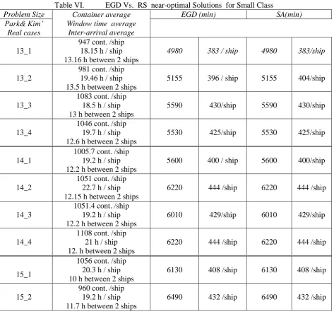
www.ijaera.org 2016, IJA-ERA - All Rights Reserved 282 Table VI. EGD Vs. RS near-optimal Solutions for Small Class
Problem Size Container average Window time average
Inter-arrival average
EGD (min) SA(min) Park& Kim’
Real cases
13_1
947 cont. /ship 18.15 h / ship 13.16 h between 2 ships
4980 383 / ship 4980 383/ship
13_2
981 cont. /ship 19.46 h / ship 13.5 h between 2 ships
5155 396 / ship 5155 404/ship
13_3
1083 cont. /ship 18.5 h / ship 13 h between 2 ships
5590 430/ship 5590 430/ship
13_4
1046 cont. /ship 19.7 h / ship 12.6 h between 2 ships
5530 425/ship 5530 425/ship
14_1
1005.7 cont. /ship 19.2 h / ship 12.2 h between 2 ships
5600 400 / ship 5600 400/ship
14_2
1051 cont. /ship 22.7 h / ship 12.15 h between 2 ships
6220 444 /ship 6220 444 /ship
14_3
1051.4 cont. /ship 19.2 h / ship 12.2 h between 2 ships
6010 429/ship 6010 429/ship
14_4
1108 cont. /ship 21 h / ship 12. h between 2 ships
6220 444 /ship 6220 444 /ship
15_1
1056 cont. /ship 20.3 h / ship 10 h between 2 ships
6130 408 /ship 6130 408 /ship
15_2
960 cont. /ship 19.2 h / ship 11.7 h between 2 ships
6490 432 /ship 6490 432 /ship
The results shown in Tables (7, 8 and 9) are the best results found by each of the algorithm after several trials and after the parameters tuning. We conclude that the EGD outperforms SA in several cases for medium and large instances. Even if the two algorithms find the same solution (for small class), EGD is doing that in less iterations than SA.
The number of iterations was the same for each instance solved by EGD or SA and set between 2.105 (for Small Class) and 2.5.105 (for Medium Class). For large generated size problems, this number is set between 3.5.105 and 4.105.
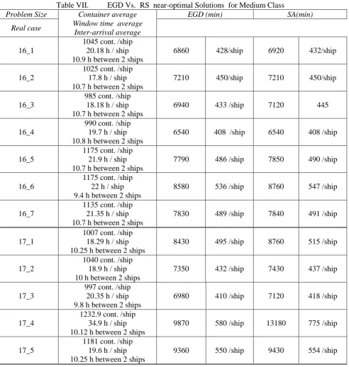
www.ijaera.org 2016, IJA-ERA - All Rights Reserved 283 Table VII. EGD Vs. RS near-optimal Solutions for Medium Class
Problem Size Container average Window time average
Inter-arrival average
EGD (min) SA(min)
Real case
16_1
1045 cont. /ship 20.18 h / ship 10.9 h between 2 ships
6860 428/ship 6920 432/ship
16_2
1025 cont. /ship 17.8 h / ship 10.7 h between 2 ships
7210 450/ship 7210 450/ship
16_3
985 cont. /ship 18.18 h / ship 10.7 h between 2 ships
6940 433 /ship 7120 445
16_4
990 cont. /ship 19.7 h / ship 10.8 h between 2 ships
6540 408 /ship 6540 408 /ship
16_5
1175 cont. /ship 21.9 h / ship 10.7 h between 2 ships
7790 486 /ship 7850 490 /ship
16_6
1175 cont. /ship 22 h / ship 9.4 h between 2 ships
8580 536 /ship 8760 547 /ship
16_7
1135 cont. /ship 21.35 h / ship 10.7 h between 2 ships
7830 489 /ship 7840 491 /ship
17_1
1007 cont. /ship 18.29 h / ship 10.25 h between 2 ships
8430 495 /ship 8760 515 /ship
17_2
1040 cont. /ship 18.9 h / ship 10 h between 2 ships
7350 432 /ship 7430 437 /ship
17_3
997 cont. /ship 20.35 h / ship 9.8 h between 2 ships
6980 410 /ship 7120 418 /ship
17_4
1232.9 cont. /ship 34.9 h / ship 10.12 h between 2 ships
9870 580 /ship 13180 775 /ship
17_5
1181 cont. /ship 19.6 h / ship 10.25 h between 2 ships
9360 550 /ship 9430 554 /ship
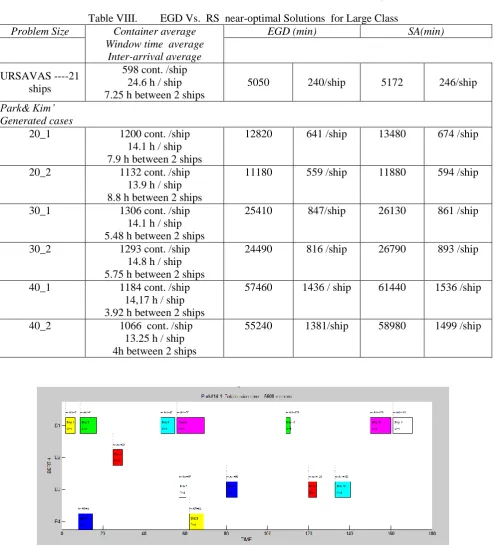
www.ijaera.org 2016, IJA-ERA - All Rights Reserved 284 Table VIII. EGD Vs. RS near-optimal Solutions for Large Class
Problem Size Container average Window time average
Inter-arrival average
EGD (min) SA(min)
URSAVAS ----21 ships
598 cont. /ship 24.6 h / ship 7.25 h between 2 ships
5050 240/ship 5172 246/ship
Park& Kim’ Generated cases
20_1 1200 cont. /ship 14.1 h / ship 7.9 h between 2 ships
12820 641 /ship 13480 674 /ship
20_2 1132 cont. /ship 13.9 h / ship 8.8 h between 2 ships
11180 559 /ship 11880 594 /ship
30_1 1306 cont. /ship 14.1 h / ship 5.48 h between 2 ships
25410 847/ship 26130 861 /ship
30_2 1293 cont. /ship 14.8 h / ship 5.75 h between 2 ships
24490 816 /ship 26790 893 /ship
40_1 1184 cont. /ship 14,17 h / ship 3.92 h between 2 ships
57460 1436 / ship 61440 1536 /ship
40_2 1066 cont. /ship 13.25 h / ship 4h between 2 ships
55240 1381/ship 58980 1499 /ship
From Tables 7, 8 and 9, we can notice the important influence of the parameter inter-arrival time on the output. In fact the total service time is more sensitive to the inter-arrival time than to the service time (here the number of container on the ship). This conclusion was drawn after solving the different instances above which reveals that, for the size problem of 14, 15 and 16 ships, the maximum total service time is found for the minimum inter-arrival time average instance.
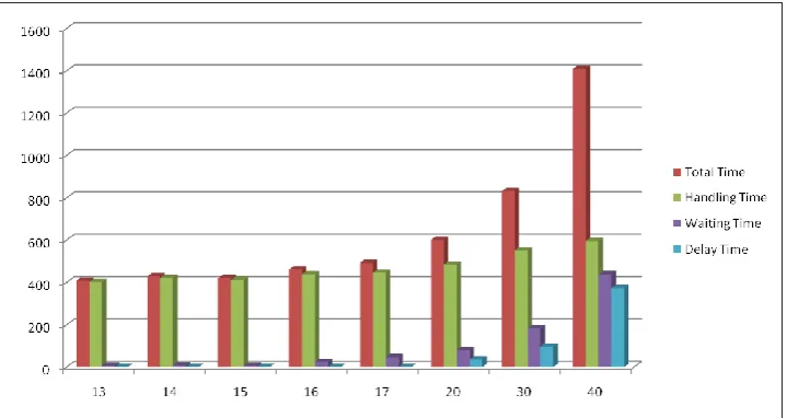
www.ijaera.org 2016, IJA-ERA - All Rights Reserved 285 depending on the size problem. In fact, we can notice that size problem has a significant effect on this total time and especially on its distribution. When the class problem is small, total time is composed almost exclusively of service time. Waiting time begins to appear in medium class problem, and for large a class, waiting time and delay are present significantly almost for all ships, and this directly impacts resolution time.
Figure 4 : Average Total time and its repartition Vs. problem size
Another interesting conclusion emerge in this study and this time, it is about the EGD meta-heuristic; we remark that the best results for the large instances (30 ships and more ) are found when using the geometric ceil decreasing such B decreases by B*(1-∆B) rather than B-∆B at each iteration. This can be seen in more details in future works.
VII. ADOPTEDAPPROACHTOSOLVETHEMULTI-OBJECTIVEPROBLEM
At a container terminal there are always two parts. Shipping lines who want their vessels to be served upon arrival and complete their loading/unloading operations within a prearranged time window and the terminal operators, who want to improve their efficiency, optimize their logistic process and the throughput of the terminal. Due to this fact, problems dealing with the container terminals generally have a multi-objective aspect to find a compromise between these two parts.
Berth allocation problem can be seen as a multi-objective problem where shipping lines seek to minimize their total service time and on another hand terminal operators have to offer their service in an optimal and efficient way.
As presented in part 3.2 in this work, the second objective formulated above, is the minimization of the workload standard deviation of cranes, considered an indicator of the efficiency of the terminal. For more details we refer the reader to [4].
www.ijaera.org 2016, IJA-ERA - All Rights Reserved 286 objectives. The particularity of that sum is that the weights are varied dynamically during the search. For more details, we refer the reader to [16].
After having implemented the algorithm presented in [16], we still have a few remarks about some shortcomings, ie, the approach is using a transformation of the different objectives into a single one but not the classical weighted technique where having necessarily the weight sum equal to 1, It ‘s difficult to choose the initial weight parameters which is, according to the authors important; and finally we think that it ‘s not always possible to set a reference solution which is , necessary to run the algorithm .
Because of the gaps in the previous algorithm, and because the EGD has not been explored thoroughly enough for the multiobjective problems, in this paper, and this is the most interesting contribution, we propose two Pareto Archived variants of EGD which were inspired from the Engrand’s Multi-Objective Simulated Annealing (MOSA) in [17] in terms of dominance principle and return to base technique. But unlike Engrand in [17] who, proposed a new function G, sum of the logarithms of the different single objective, the first variant is treating each objective separately and the second is applying the classical weighted sum, found for the most aggregated methods.
We simply called the first (PA-EGD) where each objective is evaluated separately in each iteration, then an "archive" is created to store the non dominated solutions during the search. The second is called (PA-WEGD) because it is using weights to transform the different objectives into a single one.
These two variants are based on the non dominance principle and thus are trying to find the Pareto set solutions. To simply summarize the non dominance principle, let’s assume that a reasonable solution to a multi-objective problem is to investigate a set of solutions, each of which satisfies the objectives at an acceptable level, and without being dominated by any other solution; it’s the Pareto optimal set. Consequently, a solution belongs to the Pareto set if there is no other solution that can improve at least one of the objectives without degrading any other objective.
A. Pareto Archived EGD (PA-EGD)
This algorithm is based first on the extended great deluge acceptance for neighbour solutions and secondly on the non dominance archiving principle. The algorithm also periodically executes a "return-to-base" option which continues search by selecting randomly a solution from the archive. This is done to try to ensure that the entire trade-off is found.
The PA-EGD starts by taking each objective i separately and associates a ceil Bi to each of them for the initialisation of the algorithm. Table 10 presents the proposed algorithm.
In our case, B1 is the initial total service time associated to the first solution found by the construction
heuristic and B2 is the workload standard deviation of cranes associated to this same first solution. At
www.ijaera.org 2016, IJA-ERA - All Rights Reserved 287 Table IX. : PA-EGD
B. Pareto Archived Weighted EGD (PA-WEGD)
In the last section, the multi-objective optimization algorithm is treating each objective separately. In this part, the search is based on an aggregating technique which converts the different objectives into a single one by a weighted sum [18]. The weakness of this approach s is the difficult choice of the weights in advance when we do not have enough information about the problem [18] .To palliate to this point, we have developed an algorithm trying to cover several configurations of weights. For our case, we have 2 objectives, the weighted sum can be written then as
F(s) =wf1(s) + (1-w) f2(s).
We notice here that only one parameter w, is adjusted. In fact, the weight w is initialized to 0.1 and is increased by 0.1 at each search iteration in order to realize various search directions to uncover more non-dominated solutions in the solution space.
C. Experiments and results for the Multi-objective problem
The 2 techniques PA-EGD and PA-WEGD are tested and compared for the resolution of the Multi-objective BACAP presented in [4].
The aim of this section is to apply the two above proposed EGD based algorithms on a 13 ships instance presented in Table 12 from [4], and compare the results obtained with the multi-objective hybrid genetic algorithm developed by the authors.
Set the initial solution S
Calculate initial cost functions f1(s), f2(s)
Initial ceilings B1=f(s); B2= f2(s)
Specify input parameter ∆B1; ∆B2=?
While not stopping condition do Define neighbourhood N(s)
Randomly select the candidate solution S* Є N(s)
If (f1(s*) ≤ f1(s)) or (f1(s*) ≤ B1) & (f2(s*) ≤ f2(s)) or (f2(s*) ≤ B2)
Then Accept S* Update the Archive
Do not archive S* if dominated by one archived individual, Archive S* if not dominated by any archived individual, Remove archived individual if dominated by S*
Lower the ceilings B1 = B1 - ∆B1and B2 = B2 - ∆B2
www.ijaera.org 2016, IJA-ERA - All Rights Reserved 288 Table X. : PA-EGD
Table XI. : 13 ships Instances Information from [4]
Sr. No.
Ship Name Arrival Time Due Time Total number of container
loading/unloading (TEU)
1 ZHE 01:00 17:00 525
2 ZHW 01:00 17:00 515
3 ZYE 01:00 15:00 722
4 ZYW 01:00 15:00 741
5 ZX 00:00 14:00 400
6 JWH 05:30 17:30 664
7 JYD 01:30 12:00 227
8 XNT 05:30 22:00 795
9 DY 07:54 10:25 34
10 MZ 13:54 14:59 31
11 ZH 00:00 14:30 149
12 XY 15:00 22:00 236
13 YL 20:06 23:50 105
In the following Table 13 and on the figures 5, 6, 7 and 8, the pareto solutions and the accepted solutions, found by PA-EGD and PA-WEGD are presented for both Liang’s instances with 11 and 13 ships respectively. In the second colon of the table 13, the Liang results are detailed as found by [4]. The authors choose the solutions (Z1 --- Z2) such as (55.13 --- 2.5) & (95.2 --- 2.44) as the pareto solution closest to the ideal points in both configurations with 11 and 13 ships. As presented graphically in [4], the ideal points for the 11ships instance and 13ships instance respectively are (51---1.5) and (89---1.4).
We may notice that the Pareto solutions (bold writing) found by both the PA-EGD and PA-WEGD try to reach closely the ideal points, which prove the performance of the proposed algorithms when we compare the solutions to those found by a well known multi-objective algorithm such as GA.
Set the initial solution S While 0.1≤ w ≤ 1
Calculate the initial weighted function F(s) =wf1(s) +(1-w) f2(s)
Initial ceilings B=F(s);
Specify input parameter ∆B=?
While not stopping condition do Define neighbourhood N(s)
Randomly select the candidate solution S* Є N(s)
If (F(s*) ≤ F(s)) or (F(s*) ≤ B) Then Accept S* Update the Archive
Do not archive S* if dominated by one archived individual, . Archive S* if not dominated by any archived individual, . Remove archived individual if dominated by S*
Lower the ceiling B = B - ∆B w=w+0.1
www.ijaera.org 2016, IJA-ERA - All Rights Reserved 289 The figures 5 and 7 shows the Pareto solutions (green points) and accepted solutions (blue points) during the PA-EGD search, respectively for 13 and 11 ships The space is enveloped by the two ceils (B1=Total service time on left and B2=Workload on the top ). The curve Pareto represents the non
dominated solutions.
By analogy, figures 6 and 8 shows both Pareto solutions (red points) and accepted solutions (blue points) during the PA-WEGD search, respectively for 13 and 11 ships.
Figure 5: Pareto and accepted
Solutions by PA-EGD for 13 ships
Figure 6: Pareto and accepted Solutions by PA-WEGD for 13 ships
Figure 7: Pareto and accepted Solutions by PA-EGD for 11 ships
www.ijaera.org 2016, IJA-ERA - All Rights Reserved 290 Table XII. Multiobjective Solutions for PA-EGD & PA-WEGD
Instance Pareto Solution Liang (Genetic
Algorithm)
PA-EGD
PA-WEGD
Z1 Z2 Z1 Z2 Z1 Z2
Liang-- 11 ships
51.33 51.9 53.15 55.13 57.68 60.45 62.73 4.6 4.3 3.12 2.5 1.8 1.52 1.5 38,93 41,33 42,21 42,57 46,05 46,15 47,93 48,38 48,38 50,4 50,85 56,60 57,93 8,40 6,79 5,92 4,55 4,53 4,14 3,76 3,34 3,24 2,67 1,83 1,66 0,89 38.17 40.07 42.70 43.59 46.19 47.86 49.97 51.38 52.15 55.84 54.62 55.18 58.20 61.73 68.12 72.84 73.15 97.35 11.39 11.17 9.09 6.24 5.82 4.81 4.11 3.57 2.57 2.41 1.87 1.80 0.72 0.61 0.56 0.38 0.23 0.16 Liang--13 ships 90.32 91.67 91.8 1.87 93.33 94.17 95.2 103.47 114.75 130.23 134.70 142.57 152.82 171.48 5.6 5.13 3.68 4.62 3.98 3 2.44 2.34 1.98 1.59 1.48 1.47 1.46 1.36 94.06 94.38 95.30 103.22 110.68 111.01 111.23 111.98 127.90 139.33 139.68 113.03 1.64 1.49 1.29 0.90 0.74 0.71 0.68 0.39 0.15 0.12 0.06 0.26 90,02 92,04 95,66 102,74 104,85 105,18 115,15 117,67 117,68 5,73 1,73 1,31 1,14 0,99 0,40 0,29 0,19 0,16 VIII. CONCLUSION
In this paper we have attempted to solve a BACAP in its discrete-dynamic variant in both mono-objective and multi-mono-objective cases. The approach chosen is based on an extended Great Deluge meta-heuristic preceded by a meta-heuristic to construct the initial feasible solution. The approach has exploited the inherent advantages with this Extended Great Deluge technique in escaping from local optima while also maintaining a relatively simple set of neighborhood moves. The results found in this paper could be compared to others meta-heuristics solutions.
www.ijaera.org 2016, IJA-ERA - All Rights Reserved 291 to solve the problem for medium and large case problems taken from an adapted (slightly revisited to fit the problem) BACAP benchmark [1]. In both cases, the performance of the algorithm has been demonstrated.
In this work, and for large instances, another way to decrease the ceil B in the EGD has been tested and proved to be efficient.
We have also concluded in this work, that for the issue treated, inter-arrival time is the most influent parameter and that the problem size affects the complexity of the resolution and thus resolution time.
The two proposed algorithms developed for the multi-objective problems, named EGD and PA-WEGD are subject to be more thoroughly studied for other kind of problems in the future.
Conflict of interest: The authors declare that they have no conflict of interest.
Ethical statement: The authors declare that they have followed ethical responsibilities
REFERENCES
[1] Park, Y.M., Kim, K.H., “ A scheduling method for Berth and Quay cranes, ” Operational Research Spectrum, vol. 25, 2003, pp. 1-23
[2] Miesel, F., and Bierwirth ,C., “Integration of Berth Allocation and Crane Assignment to Improve the Resource Utilization at a Seaport Container Terminal, ”. Operations Research Proceedings , 2006. [3] Liang, C., Huang, Y., Yang, Y. , “ A quay crane dynamic scheduling problem by hybrid evolutionary
algorithm for berth allocation planning, ” Computers and Industrial Engineering. 2009, vol. 56. No. 3, pp. 1021-1028.
[4] Liang ,C.,Lin,L.,Jo,J. , “Multiobjective hybrid genetic algorithm for quay crane scheduling in berth allocation planning .’’, Intell. J. Manufacturing Tecnology and Management., 2009, vol.16. No.1/2. [5] Imai, A., Chen, H.C., Nishimura, E., Papadimitriou, S., “ The simultaneous berth and quay crane
allocation problem, ” Transportation Research Part E, vol.44 (5), 2008, pp. 900-920.
[6] Bierwirth, C., Meisel, F., ‘’A follow survey of berth allocation and crane scheduling problems in container terminals. European Journal of Operational Research. 1-15.
[7] Meisel, F., Bierwirth, C., “ Heuristics for the integration of crane productivity in the berth allocation problem, ” Transportation Research Part E, vol. 45 (1), 2009, pp.196–209.
[8] Bierwirth, C., Meisel, F., “A survey of berth allocation and quay crane scheduling problems in container terminals, ” European Journal of Operational research. No. 202, 2010, pp. 615-627.
[9] Cordeau,J.F, Laporte,J., Legato,P., Moccia,L., 2005. ‘’Models and tabu search heuristics for the berth allocation problem’’. Transportation Science. vol.39.
[10] Cheong and Tan, ‘’A multi-objective multi-colony ant algorithm for solving berth allocation problem’’ . Y. Liu, A. Sun, H.T. Loh, W.F. Lu, E.-P. Lim (Eds.), Advances of Computational Intelligence in Industrial Systems, Springer-Verlag, Berlin (2008), pp. 333–350.
[11] Kim,K.H., Moon , ‘’Berth scheduling by Simulated Annealing’’. Transportation Research Part B vol. 37 pp. 541–560.
[12] Lee.Y, Chen,C.Y.,’’ An optimization heuristic for the berth scheduling problem, European Journal of Operational Research 196 (2009) 500–508.
[13] Lin,S.W, Ying,K.C,, and Wan,S.Y , “Minimizing the Total Service Time of Discrete Dynamic Berth Allocation Problem by an Iterated Greedy Heuristic,” The Scientific World Journal, vol. 2014, Article ID 218925, 12 pages, 2014.
[14] Burke E.K., Y. Bykov, J.P. Newall and S. Petrovic, “A Time-predefined local search approach to exam timetabeling problems, ” IIE Transactions, vol. 36 (6), 2004, pp. 509-528.
www.ijaera.org 2016, IJA-ERA - All Rights Reserved 292 [16] Petrovic, S., Bykov, Y. A Multiobjective Optimisation Technique for Exam Timetabling Based on
Trajectories
[17] Engrand. P. (1997). A multi-objective approach based on simulated annealing and its application to nuclear fuel management. 5th Inter. Conference on Nuclear Engineering, Nice, France, pp. 416 -423. [18] C. A. Coello Coello, “An updated survey of evolutionary multiobjective optimization techniques: State
of art and future trends,” in Proceedings, Congress on Evolutionary Computation, 1999, pp.3-13.