Using of Artificial Neural Networks to Recognize the Noisy Accidents Patterns of Nuclear Research Reactors

(1)

Using of Artificial Neural Networks to

Recognize the Noisy Accidents Patterns of

Nuclear Research Reactors

Eng. Abdelfattah A. Ahmed

Atomic Energy Authority, Nuclear Research Center, Inshas, Egypt Email: [email protected].

Prof. Dr. Nwal Ahmed Alfishawy

Minufiya University, Faculty of Electronic Engineering, Minuf, Egypt. Prof. Dr. Ali Karam Eldin

Atomic Energy Authority, Nuclear Research Center, Inshas, Egypt Dr. Said Sh. Haggag.

Atomic Energy Authority, Nuclear Research Center, Inshas, Egypt

---ABSTRACT--- In this paper, an approach based on neural networks for recognizing the nuclear research reactor accidents (patterns) is presented. A neural network is designed and trained, initially without noise, to recognize the nuclear research reactors accidents patterns (using MATLAB's Neural Network Toolbox). When the neural network response is simulated, the 9x9 simulation output values of the matrix's diagonal is larger than 0.9, (approximately equal 1), this means the outputs is approximately equal the targets and the network is well trained. A new copy of the neural network was made, to train it with noisy accident's patterns. When this network was trained on this noisy input vectors (patterns), it is greatly reduces its errors and its output is approximately equal the output as when it is trained without noise input vectors. This new copy was trained also on accidents patterns without noise to gain the maximum performance and the high reliability of the network. Experiments have shown excellent results; where the network did not make any errors for input vectors (patterns) with noise level from 0.00 up to 0.14. When the noise level larger than 0.15 was added to the vectors (patterns); both neural networks began making errors

Keywords:

Artificial neural networks (ANN), Nuclear Research Reactor, and MAT

--- Date of Submission: June 13, 2011 Date of Acceptance: August 17, 2011 ---

1. Introduction

A

n Artificial neural network is defined as an assembly of interconnected processing elements used to represent a real world system, i.e. a neural network is an interconnected web of individual neurons. In simpler terms, a neural network is a mathematical system used to approximate a system output based on a specific input. Or, it is a massively parallel distributed processor made up of simple processing units, which has a natural propensity for storing experiential knowledge and making it available for use [6].

Matlab's Neural Network Toolbox is software that provides comprehensive support for many proven network paradigms, as well as graphical user interfaces (GUIs) that enable to design and manage neural networks. The Toolbox supports both supervised and unsupervised neural networks. The supervised neural networks are trained to produce desired outputs in response to sample inputs, making them particularly well suited to modeling and controlling dynamic systems, recognizing noisy data, and predicting a future event, which is our domain, demand [5-8].

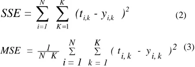
In this work, a neural network is designed and trained to recognize the 9 accidents of the nuclear reactors. By the aid of reactor operation crew and Safety Analysis Report (SAR) of the reactor, also the Atomic Energy Authority (AEA) experts, data sets was collected for the eight accidental cases listed below plus the normal operation case (Classes) as shown in Figure (1). So the total cases, which we have, are nine. The result is that each accident is represented as a 3-by-5 grid of Boolean values.

(2)

However, the data sets perhaps are not perfect, and the accidents can suffer from noise. Perfect recognition of ideal input vectors is required and reasonably accurate recognition of noisy vectors, see Figure (2).

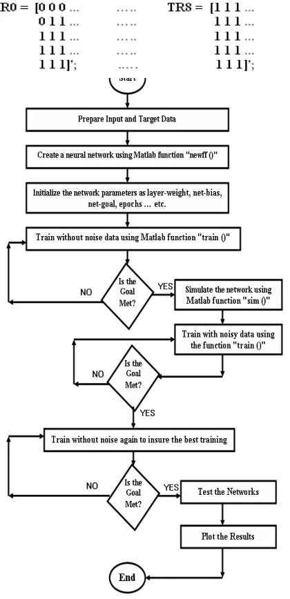
The nine 15-element input vectors are defined in the function accmodels as a matrix of input vectors called accidents. The target vectors are also defined in this file with a variable called, targets. Each input vector is a 15-element vector (3-by-5), Figure (3), with a 1 in the position of the accident it represents, and 0’s everywhere else. For example, the TR0 is to be represented by a 1 in the first element (as TR0 is the first accident of the accidents), and 0’s in elements two through fifteen. Fig. (2): Program flowchart using Matlab.

Fig. (3): Samples of (15x9) matrix of (3x5) bit maps for each Accident.

This paper comprises five sections. After this introductory section, Neural Network Implementation is in section (2). Results and Discussions are in section (3). Conclusion is in section (4). Finally, References are in section (5).

2. ANN Implementation

The network receives the 15 Boolean values as a 15-element input vector (3-by-5). It is then required to identify the accident by responding with a 9-element output vector. The 9 elements of the output vector each represent an accident. To operate correctly, the network should respond with a 1 in the position of the accident being presented to the network. All other values in the output vector should be 0.

In addition, the network should be able to handle noise. In practice, the network does not receive a perfect Boolean vector as input. Specifically, the network should make as few mistakes as possible when recognizing vectors with noise of mean 0 and standard deviation of 0.2 or less.

2.1 ANN Architecture

The neural network needs 15 inputs and 9 neurons in its output layer to identify the accidents. The network is a two-layer sigmoid/sigmoid network. The log-sigmoid transfer function was picked because its output range (0 to 1) is perfect for learning to output Boolean values.

Fig. (4): neural network design for accidents patterns recognition

a2 = f2 ( LW2,1 ( f1 ( LW1,1p + b1 ) + b2) = yj ,

where j is neurons in the output layer,

The hidden (first) layer has 10 neurons. This number was picked by guesswork and experience. If the network has trouble learning, then neurons can be added to this layer, Figure (4).

(3)

output vector with 0’s. However, noisy input vectors can result in the network’s not creating perfect 1’s and 0’s. After the network is trained the output is passed through the competitive transfer function compet. This makes sure that the output corresponding to the accident most like the noisy input vector takes on a value of 1, and all others have a value of 0. The result of this post-processing is the output that is actually used.

2.2 ANN Training

To create a network that can handle noisy input vectors, it is best to train the network on both ideal and noisy vectors. To do this, the network is first trained on ideal vectors until it has a low sum squared error. Then the network is trained on 10 sets of ideal and noisy vectors. The network is trained on two copies of the noise-free accidents at the same time as it is trained on noisy vectors. The two copies of the noise-free accidents are used to maintain the network’s ability to recognize ideal input vectors.

Unfortunately, after the training described above the network might have learned to recognize some difficult noisy vectors at the expense of properly recognizing a noise-free vector. Therefore, the network is again trained on just ideal vectors. This ensures that the network responds perfectly when presented with an ideal accident. All training is done using backpropagation with both adaptive learning rate and momentum, with the function 'traingdx'. The Error (Performance) is calculated in terms of Sum-Squared Error (SSE), equation (2), or Mean-Squared Error (MSE), equation (3), according to the choice of the performance function at the network creation by the following two equations:

1 2 k i, k i, K K N 1 = i

)

y

-(t

=

SSE

∑

= (2) 2 k i, k i, K 1 = k N K

N1 (t - y )

1 = i =

MSE ∑ ∑ (3)

Where N and K denote the number of patterns and output nodes used in the training respectively, i denotes the index of the input pattern (vector), k denotes the index of the output node, ti,kand yi,kexpress the desired output

(target) and actual output values of the k

th

output node at i

th

input pattern, respectively. The calculation of the output is according to figure (4) for two layers network using equation (1).

2.2.1 Training without Noise

The network is initially trained without noise for a maximum of 5000 epochs or until the network sum squared error falls beneath 0.1. Figure (5) show the output every 20 epochs, and the training stop when the Performance goal is met at epoch number158. The

procedure for backpropagation training is as follows, (for each input vector associate a target output vector): while not STOP

STOP=TRUE for each input vector

perform a forward sweep to find the actual output obtain an error vector by comparing the actual and target output

if the actual output is not within tolerance set STOP= FALSE

perform a backward sweep of the error vector use the backward sweep to determine weight changes

update weights end while

Fig. (5): neural network training output

(4)

Fig. (7-a)

Fig. (7-b)

Fig. (7): neural network output for Accidents Patterns Recognition

2.2.2 Training with Noise

To obtain a network not sensitive to noise, a new copy of the neural network was made. This network trained with two ideal copies and two noisy copies of the vectors of accidents. The target vectors consist also of four copies of the vectors in target. The noisy vectors have noise of mean 0.1 and 0.2 added to them. This forces the neuron to learn how to properly identify noisy accidents, while requiring that it can still respond well to ideal vectors. P = [(P + randn(R,Q)* noise percent%)] (4)

To train with noise, the maximum number of epochs is reduced to 300 and the error goal is increased to 0.6, reflecting that higher error is expected because more vectors (including some with noise), are being presented 2.3.2.1 Results of training with noise

An example of the ten passes, for training the network with noise shown in the following paragraphs. In pass2, as example, the goal is met after 5 epochs, where it means one of the stopping criteria is met. The stopping criterion here is the sum of squares errors (SSE).

Pass = 2

traingdx-calcgrad, Epoch 0/300, SSE 0.67199/0.6, Gradient 1.35261/1e-006

traingdx, Performance goal met, Figure (8).

Fig. (8): training with noise (Pass2)

Fig. (9): training with noise (Pass4) Pass = 4

traingdx, Performance goal met. Figure (9).

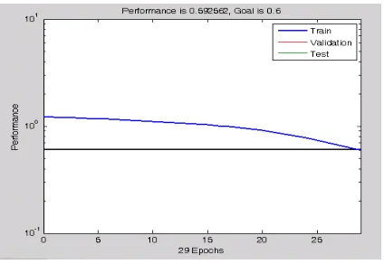
Pass = 7

(5)

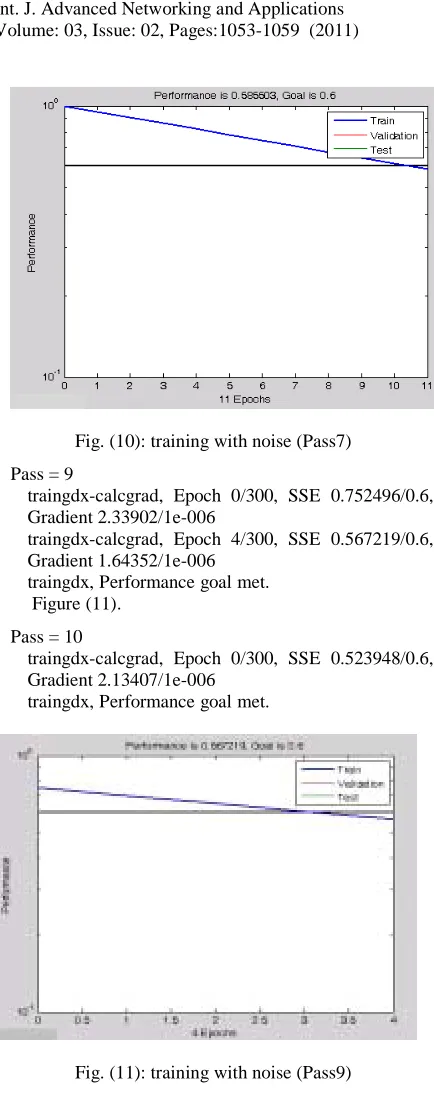
Fig. (10): training with noise (Pass7) Pass = 9

traingdx, Performance goal met. Figure (11).

Pass = 10

traingdx, Performance goal met.

Fig. (11): training with noise (Pass9) 2.2.3 Training without Noise Again

Once the network is trained with noise, it makes

sense to train it without noise once more to

ensure that ideal input vectors are always

classified correctly. Therefore, the network is

again trained with code identical to the previous

paragraph 2.3.1.

3.0 Results and Discussion

The reliability of the neural network accidents recognition system is measured by testing the network with input vectors with varying quantities of noise. The script file AccidentsRecogniton tests the network at various noise levels, and then graphs the percentage of network errors versus noise. Noise with a mean of 0 and a standard deviation from 0 to 0.5 is added to input vectors. At each noise level, 100 presentations of different noisy versions of each accident are made and the network’s output is calculated.

Fig. (12): the reliability for the network trained with and without noise

In Figure (12), the solid line on the graph shows the reliability for the network trained with and without noise. The reliability of the same network when it was only trained without noise is shown with a dashed line. Thus, training the network on noisy input vectors greatly reduces its errors when it has to recognize noisy vectors and its output is approximately equal the training the same network without noisy input vectors output.

The network did not make any errors for vectors with noise level of mean 0.00 or 0.14. When noise level of mean is larger than 0.15 was added to the vectors both networks began making errors.

If a higher accuracy is needed, the network can be trained for a longer time, or retrained with more neurons in its hidden layer. Also, the resolution of the input vectors can be increased to a 6-by-10 grid. Finally, the network could be trained on input vectors with greater amounts of noise if greater reliability were needed for higher levels of noise.

(6)

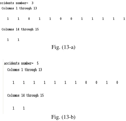
accident TR2 in figures (1), that means the network functioned correctly as expected. Also, when the same test carried out using accident TR4 and TR7, as examples, the same results were given; see figures (13-b) and all other examples were tested.

Fig. (13-a)

Fig. (13-b)

Figure (13): Sample Output of the system test when presenting sample of noisy input patterns to the neural

network

The performance of a constructed network can be measured by investigating the network response in more detail, by performing a regression analysis between the network response and the corresponding targets. Where the entire data set are entered the network and a linear regression between the network outputs and the corresponding targets are performed. After the network output and the corresponding targets are passed to the Matlab's function 'postreg', it returns three parameters for the equation:

Output = m Target + b (5)

Figure (12) illustrates the graphical output provided by the function 'postreg'. The network outputs are plotted versus the targets as open circles. The best linear fit is indicated by a dashed line. The perfect fit (output equal to targets) is indicated by the solid line. In this figure, it is difficult to distinguish the best linear fit line from the perfect fit line because the fit is so good.

Output = 0.97 Target + 0.0073 (6)

From equation (6), the first parameter is the slope m=0.97, and the second one is the y-intercept b=0.0073 of the best linear regression relating targets to network outputs. This output, you can see that the numbers are very close to the perfect fit (outputs exactly equal to targets), would be 1, and the y-intercept would be 0.

The third parameter returned is the correlation coefficient (R-value) between the outputs and targets. The correlation coefficient between two variables is a real number (r) which expresses the type and the degree of the relation between the two variables. It is a measure of how well the variation in the output is explained by the targets. If this number is equal to 1, then there is perfect correlation between targets and outputs. In the application, the number is very close to 1 (0.99953), which indicates a good fit.

Fig. (13): the reliability for the network trained with and without noise.

4.0 Conclusion

This paper proved the efficient use of an artificial neural network as a promising method for the nuclear reactor accidents patterns recognition. A two layers feedforward neural network with backpropagation training algorithm, which updates the network weights and biases in the direction of the negative of the gradient and trained with an adaptive learning rate combined with momentum training, Matlab's training function 'tringdx', is an efficient ANN to recognize the nuclear reactor accidents patterns. By testing the network with input vectors with varying values of noise, the network did not make any errors for vectors with noise level of mean 0.00 to 0.14. When noise level of mean is larger than 0.15 was added to the vectors both networks began making errors, and the network still recognize the reactor accidents patterns.

(7)

References

[01] S. Sh. Haggag, PhD Thesis, "Design and FPGA-Implementation of Multilayer Neural Networks With On-chip Learning", Atomic Energy Authority, Egypt 2nd Research Reactor. PhD, Menufia University, 2008.

[02] The International Atomic Energy Agency (IAEA) Safety Series, Vienna, "Safety in the Utilization and Modification of Research Reactors", Printed by the IAEA in Austria, December 1994, STI/PUB/961.

[03] J. Korbicz, Z. Kowalczuk, J. M. Koscielny, W. Cholewa : "Fault diagnosis: models, artificial intelligence, applications", (ISBN 3-540-40767-7, Springer-Verlag Berlin Heidelberg 2004).

[04] B. Ch. Hwang, "Fault Detection and Diagnosis of a Nuclear Power Plant Using Artificial Neural Networks", (Simon Fraser University, March 1993).

[05] A. Bartkowiak, "Neural Networks and Pattern Recognition", (Institute of Computer Science, University of WrocÃlaw, 2004).

[06] M. T. Hagan, H. B. Demuth, "Neural Network Design", (PWS Publishing Company, a division of Thomson Learning. United States of America, 1996).

[07] S. Samarasinghe "Neural Networks for Applied Sciences and Engineering: From Fundamentals to Complex Pattern Recognition", (Publisher Auerbach Publishing, ISBN-10: 0-8493-3375-X, Taylor & Francis Group, LLC, 2006).