The Optimized Three-Dimensional Deployment for
Pipeline Systems in Wireless Sensor Networks
Huaping Yu
College of Computer Science, Yangtze University, Jingzhou, China Email: [email protected]
Lan Huang
College of Computer Science, Yangtze University, Jingzhou, China Email: [email protected]
Abstract—Pipeline systems are vital infrastructure to national economy, and are widely used for transporting liquid and gas matter, such as oil, natural gas, water and chemic materials. However, effective and efficient management of pipeline systems are challenging, due to its mere lengths and the diverse deployment environments. Wireless sensor network (WSN) consists of a large number of sensors, which can automatically and constantly collect and transmit monitored data, and thus can enable effective and timely management of pipeline systems. Successful WSNs rely on the deployment of sensor nodes. Most current research assumes that sensor nodes are deployed on a two-dimensional plane. However, in reality, sensor nodes deployed on pipeline surface exist in a three-dimensional space. In this paper, we present an optimized 3D deployment model of WSN particularly for pipeline systems. The model is based on analyzing various relationships between sensing ranges of sensor nodes and pipeline radii. We also provide an efficient deployment algorithm based on the model. Empirical simulation results show that the proposed model and the algorithm can provide both theoretical guidance and practical basis for the three-dimensional deployment of sensor nodes in pipeline systems.
Index Terms—three-dimensional deployment, pipeline system, hierarchical network architecture
I. INTRODUCTION
Wireless sensor networks (WSNs) are networks that consist of a large number of resource-limited sensor nodes. Each node is typically equipped with sensors of different types, computational units, storage devices and communication modules. These components, as a whole, can automatically sense, process, and transmit all kind of monitored data, without any human intervention. Therefore, WSNs already have many civil and military applications, such as health-care[1], environmental monitoring [2], scientific exploration[3], battlefield surveillance[4] , etc.
Transmission pipelines are vital infrastructure to national economy. Such pipelines are widely used for
transporting large quantities of liquid and gas matter, such as crude oil, natural gas, water and chemic materials, due to its lower long-term costs, higher capacity and better consistency than alternative transporting methods such as railroad and highway. However, managing transmission pipelines is challenging, especially with the rapid growth in the length of the pipelines. Successful pipeline management must monitor leak, pressure, flow, corrosion, pollution in surrounding environment, and many other factors that can affect the safety of the pipelines and thus transportation efficiency. WSNs can be used to ensure the efficiency and safety of pipeline without costly expansion [5], which can effectively improve the level of management.
Successful application of WSNs relies on the deployment of sensor nodes. Recent research on sensor node deployment mainly focus on two-dimensional models—how to effectively and efficiently set up sensor nodes in a two-dimensional plane [6-9]. However, in reality, sensor nodes deployed on pipeline surface exists in a three-dimensional space. Although there exists some research on deployment models of sensor nodes in 3D space, few can be applied to the context of pipeline systems. In this paper, we study this problem—optimized sensor node deployment in a three-dimensional space— specifically for pipelines.
The rest of this paper is organized as follows. Next, we discuss related work. Then we describe the geometric structure of a pipeline and the typical three-tier-network architecture for WSNs. Section IV presents the new 3D sensor node deployment model for pipelines and its implementation algorithm, based on the analysis of the geometric relationships between sensor node’s sensing ranges and the radius of a pipeline. Section V analyzes the empirical simulation results, from connectivity, coverage and energy consumption respectively. Section VI concludes the paper.
II. RELATED WORK
Maximizing sensing coverage efficiency is a fundamental and critical issue for successful WSN applications. In recent years, the coverage problem has been extensively studied in the context of two-dimensional planes [6-9]. However, in reality, sensor
Project number: PetroChina Innovation Foundation (Grant No. 2013D-5006-0605).
nodes embedded in the real physical world exist in three-dimensional space. Recently, there has been increasing research on 3D deployment models [10, 11, 12, 13, 14, 15, 16, 17]. Given a long-narrow region, Zhou[10] analyzes the basic requirements for optimal deployment of nodes in all directions, designs a 3D linear node deployment strategy adapted to fault coverage and proposes an energy-efficient network zoning strategy under fault-tolerant coverage. Liu [11] provides a new lattice-based technique for topology construction in 3D WSNs. Jiang and Liu [12] propose a energy-aware coverage algorithm that takes coverage ratio into account also for 3D WSNs. Zhang, Yu and Zhang [13] propose a distributed energy efficient 3D coverage control algorithm. Li, Feng and Hou [14] transfer their 2D algorithm SGA (Stand Guard Algorithm) to 3D, based on the characteristics of the 3D space. Li and Liu [15] propose a novel three-dimensional grid model algorithm MCC3D (Max Coverage Connectivity 3D). Ammari and Das [16] discuss the connectivity and k-coverage issues in 3D WSNs and propose the reuleaux tetrahedron model to characterize k-coverage of a 3D field and investigate the corresponding minimum sensor spatial density. Pompili, Melodia and Akyildiz [17] study the deployment strategies for two-dimensional and three-two-dimensional communication architectures for underwater acoustic sensor networks
Node deployment methods can be classified into two types: random deployment and deterministic deployment. Pipeline coverage—the problem we consider in this paper—belongs to the latter. None of the related research discussed above considers the structure characteristics of the pipelines, for example, their radius and lengths. However, these are the primary factors that can affect coverage efficiency. Consequently, in this research, we take the relationship between pipeline radius and sensor nodes’ sensing ranges into account.
III. SYSTEM ARCHITECTURE AND THREE-DIMENSIONAL
SENSOR NODE DEPLOYMENT BASED ON WSNS
In this section, we describe the pipeline architecture and the typical 3-tier deployment structure of WSNs. These form the basis of our 3D sensor node deployment model, which will be explained in details in the next section.
A. Architecture of a Pipeline
Pipelines are made from steel or plastic tubes with an inner diameter typically ranging from 0.1m to 5m [18]. Figure 1 (a) shows the architecture of a standard pipeline. We project the 3D pipeline structure into two 2D planes-the XY plane and planes-the XZ plane, as shown in Figure 1 (b), with r being the radius and L the length of the pipeline. Wireless sensor nodes can only be deployed on the pipeline wall. This means that in the XY-projected topological graph, all sensor nodes exist on the edge of the circle, whereas in the XZ-projected graph they are located on the two longer edges of the rectangle, and inside the rectangle.
y X
z
x
2r r
L
XY plane projection
XZ plane projection
z
Y
L x
o
(a) (b)
Pipeline Sensor Node
Figure 1. The pipeline architecture
B. Three-tiers Network Architecture for Pipeline System Based on WSNs
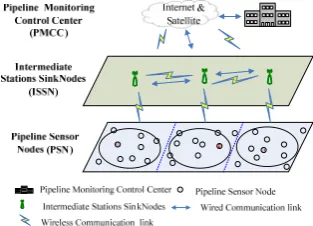
A WSN-based pipeline monitoring network typically consists of three tiers: the pipeline sensor nodes (PSNs) at the bottom, the intermediate stations sink nodes (ISSNs) and the pipeline monitoring control center (PMCC) at the top, as shown in Figure 2 [19].
Figure 2. The network architecture of pipeline system based on WSNs
PSNs, i.e. the sensor nodes, deployed on the pipeline surface, sense pipeline state information in real time, such as pressure, quantity of flow, pipeline leak, pipeline corrosion, wax precipitation, environmental pollution and weather information. Each PSN has restricted computing and storage capability and limited battery, which cannot be recharged. Therefore, it is important that the sensor nodes deployment must be energy-efficient so as to prolong system lifetime.
In the middle tier, ISSNs are installed at initial injection station, compressor or pump station, partial delivery station, valve station and final delivery station [18]. The deployment is shown in Figure 3. Each ISSN has abundant computing and storage resource compared to PSNs. Furthermore, ISSNs can be recharged in time. The main functions of ISSNs include analyzing data from PSNs and uploading the data to pipeline monitoring control center (PMCC). ISSNs form a middle tier network via satellite or Internet communication.
Figure 3. The deployment of PSNs and ISSNs
forming the overall analysis and issuing the information to managers.
IV. THE THREE-DIMENSIONAL DEPLOYMENT OF PIPELINE
SENSOR NODES
As discussed before, successful application of WSNs rely on the effective deployment of sensor nodes: they must form a comprehensive and seamless coverage of the pipeline so that sensing information is complete and accurate. Meanwhile, because PSNs-sensor nodes for pipelines—are placed determinately and permanently, methods for finding their optimal positions on the pipeline surfaces are essential to PSN deployment.
Given r the radius of the pipeline and rsthe sensing range of a sensor node, there can be four possible relationships between r and rs: rs≥2r, 2r≤rs<2r, r≤
rs< 2r and rs <r. Different rsmeans different sensing coverage of the sensor node. Therefore, we analyze the optimal deployment model for each of the four rs ranges. We first determine the deployment model in the XY plane, and then expand it to the Z axis direction.
A. rs≥2r
Figure 4 shows the sensing coverage of the sense node in blue dotted circle and the pipeline in black circle. Given a point A(xs,ys) on the sensing surface and a point B(xp,yp) on the pipeline surface, we can easily derive the following equations between the two points’ coordinates and the radii r and rs:
θ
θ
2
sin
sin
r
r
x
s=
s≥
,
y
s=
r
ssin
θ
(1)
θ
θ
θ
2 sin cos 2sin r
r
xp= =
,
y
p=
r
+
r
cos
θ
(2)
θ
θ
2 ( , )
s sy
x ) , (xp yp
θ θ
2
) , (xsys
) , (xpyp
Figure 4. Sensing coverage in the XY plane whenrs≥2r
Because cosθ≤ ,1θ∈[0,π/4],r>0 , we get equation (3), which indicates that a single sense node can cover the pipeline completely.
s
p r r x
x =2 sin
θ
cosθ
≤2 sinθ
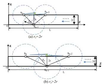
≤(3) Figure 5 illustrates the seamless coverage in the XZ plane while rs
≥
2r. This can further be classified into two cases: rs=2r and rs>2r. In either case, the distance between two closest sensor nodes on the same side of the pipeline Sn and Sn-2 is) 4 (
2 |
| 2 2
2 r r r
S
Sn n− = s+ s −
(4) When rs is greater than 2r, |SnSn-2| is greater than 2rs, which means the sensor node placed between Sn and Sn-2 but on the opposite side can provide partial coverage, as shown in Figure 5(b).
2r
sn
sn-1
2r
rs
sn-2
x
L
z
O
2r
sn
sn-1
2r
rs
sn-2
x
L
z
O
(a) rs=2r
(b)rs>2r
Figure 5. Sensing coverage in the XZ plane whenrs≥2r
B. 2r≤rs<2r
When 2r≤rs<2r, as shown in Figure 6, a single node cannot provide full coverage, but two nodes can do when placed properly. Let A, B denote the intersection points between the sensing ranges of two sense nodes deployed on the opposite side of the pipeline with the same Z position, i.e. one on O and one on D in figure 6. It is clear that as long as |BC|≥r, that is, when rs≥ 2r, two sensor nodes placed opposite each other can provide seamless coverage of the pipeline.
r
rs= 2 2r>rs> 2r
Figure 6. Sensing coverage in the XY plane when 2r≤rs<2r
In the XZ plane, coverage model is shown in Figure 7. For clarity for analysis, two PSNs are located on the surface of the pipeline with a symmetrical way. It is clear that the distance of between two nearest PSNs on the same side of the pipeline can be expressed as follow according to the figure 7.
2 2 3 1
2| | | 2
|SnSn− = Sn−Sn− = rs −r
(5)
Figure 7. Sensing coverage in the XZ plane when 2r≤rs<2r
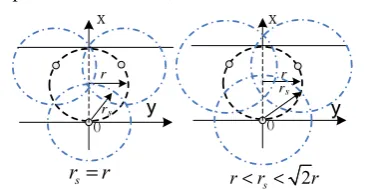
C. r≤rs< 2r
placed properly. Figure 8 shows the seamless coverage in the XY plane when r≤rs< 2r.
2 s r r< < r s
r =r
Figure 8. Sensing coverage in the XY plane whenr≤rs< 2r
In particular, Figure 9 demonstrates the seamless coverage in the XZ plane. It is clear that the distance between two nearest PSNs on the same side of the pipeline can be expressed as follow:
2 2
2 n-5 s
|Sn− S | 2= r -9/16*r
(6)
Figure 9. Sensing coverage in the XZ plane whenr≤rs< 2r
D. rs <r
In this case, the PSNs set cannot completely cover the pipeline surface in the XY plane, no matter how many PSNs are placed, as shown in figure 10.
r
rs< rs=r
Figure 10. Sensing coverage in the XY plane whenrs <r
E. Optimized 3D Deployment Algorithm
Let L denotes the length of a pipeline, on which sensor nodes are to be deployed and Ns the total number of PSNs. Then the relation between L and Ns is
2
2 / | | 1
s n n
N =⎡⎢ L S S− ⎤⎥+ , (7) according to Figures 4 and 8.
Based on previous analysis of the relationships between sensing range and the pipeline radius, the optimized algorithm for 3D deployment can be described in pseudo-code as below.
Input: pipeline parameters(r,L), effective sense radius
(rs) and communication radius (rc)
Output:the required number of sensor node (Ns), coordinate matrix P[Ns][3]. P[i][0] denotes the X axis of node Si(i=0,Ns-1), P[i][1] the Y axis and P[i][2] the Z axis.
Main()
{ int L, r, rs, rc, Ns; If (rs≥2r)
{ Num1(); //output the number of sensor node (Ns) for pipeline monitoring system
Pos1(Ns); } //output the coordinate matrix P[Ns][3] else (2r>rs≥ 2r)
{ Num2(); Pos2(Ns); } else ( 2r>rs≥r) { Num3();
Pos3(Ns); }
else printf(“These sensor nodes that locate on the surfac e of pipeline can't completely cover pipeline system while
rs<r”) // as shown in figure 10.
Num1(), Num2(), Num3() are functions for computing the numbers of sensor nodes required in different situations. They are described respectively below.
Function Num1() // output the number of sensor node (Ns), as shown in figure 4-5
{int 2 2
2
| | 2( 4 )
s n n s s
d =S S− = r + r − r ;
2 2
s s
/(r r -4r ) 1
s
N =⎡⎢L + ⎤⎥+ ; }
Function Num2() // output the number of sensor node (Ns) , as shown in figure 6-7
{int 2 2
n n-2 s
|S S | 2 r -s
d = = r ;
2 2 s
/ r -r 1
s
N =⎡⎢L ⎤⎥+ ; }
Function Num3() // output the number of sensor node (N
s) , as shown in figure 8-9
{int 2 2
n-2 n-5 s
|S S | 2 r -9/16*
s
d = = r ;
2 2
s
/ r -9/16*r 1
s
N =⎡L ⎤+
⎢ ⎥ ; }
Likewise, Pos1(), Pos2(), Pos3() are functions for computing the coordinates of the sensor nodes in different situations, and are described below.
Function Pos1(Ns) // output the coordinate matrix P[Ns] [3], as shown in figure 4-5
{int i,P[Ns][3]; For(i=1;i<=Ns;i++)
{if (i%2==0) P[i-1][0]= 2r;else P[i-1][0]=0; // the coord inate of x axis
Function Pos2(Ns) // output the coordinate matrix P[Ns] [3], as shown in figure 6-7
{int i,P[Ns][3]; For(i=1;i<=Ns;i++)
{if (i%2==0) P[i-1][0]= 2r; else P[i-1][0]=0; P[i-1][1]=0; P[i-1][2]= (i-1)* ds; }
Function Pos3(Ns) // output the coordinate matrix P[Ns] [3], as shown in figure 8-9
{int i,P[Ns][3]; For(i=1;i<=Ns;i++)
{if (i%2==0) { P[i-1][0]= 3/2r; p[i-1][1]=3r/(2 5 );
p[i-1][2]=(i-1)*ds;}
else if (i%3==0) {p[i-1][0]=0; p[i-1][1]= 0; p[i-1][2]=(i-1)*ds;}
else {P[i-1][0]=3/2r; p[i-1][1]=-3r/(2 5 );
p[i-1][2]=(i-1)*ds; } }
V. SENSOR NODES DEPLOYMENT PERFORMANCE
ANALYSIS
This section presents empirical simulated performance analysis of our sensor nodes deployment algorithm. We evaluate from three aspects: connectivity performance, coverage performance and energy consumption performance. We also adopt the line PSNs deployment strategy to avoid unbalanced energy consumption in PSNs, which can effectively prolong the life span of network.
A. Connectivity Performance
Connectivity is an important performance indicator of wireless sensor network. The connectivity model is categorized into two types: Boolean model and probabilistic model. The latter is often regarded as can better reflect the actual communication quality between nodes. Using the probabilistic model, the communication quality between sensor node i and j C(si,sj) is
) , ( R R ) , ( R ) , ( 0 0 1 ) , ( 2 c2 c1 1 ) -) , ( ( - 1 j i c j i c j i R s s d i ir j i s s d s s d R s s d e E E s s
C i j c
< ≤ < ≤ ≤ ⎪ ⎪ ⎩ ⎪⎪ ⎨ ⎧
= λ
(8)
In equation (8), denotes the communication quality from node si to sj. Rc1defines the communication range and Rc2 the maximum communication range of the node.
Ei and Eir denote the initial and the remainder energy of sensor node si respectively. The parameter λ is the degree of attenuation of signal intensity based on communication distance, and is determined by the physical properties of the sensor node. The typical value of λ is 1 [20].
The communication quality of sensor node si, according to equation (8) is
j
1/ ( 1)m ( , )
i i j
i
C m C s s
=
= −
∑
, withm being the number of communicable neighbor sensor
nodes of node si. Therefore, the network’s connection performance can be described by equation (9).
∑
= = Ns
i i s C N C 1 1
(9) Generally, rc≥2rs (rc: the communication radius of PSN) is both necessary and sufficient to ensure a complete three-dimensional coverage of a pipeline, and this implies full connectivity in the network [21]. In practice, this requirement is achievable for most pipeline system.
B. Coverage Performance
Network coverage efficiency (referred to as
τ
) is defined as the ratio of the actual coverage volume against the maximum effective volume of a sensor node, see equation (10) [10].s m s
(r )/ (r ) s
V V
τ
= (10)rs denotes the sensing radius of PSNs, Vs indicates the actual coverage volume of PSNs, and Vm denotes the max coverage volume of these PSNs.
Given a pipeline system with length L, if Ns PSNs are deployed on its surface, then
τ
is calculated as follows:2 2
3 3
S s
r 3
4N r /3 4 s s
L r L
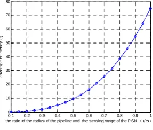
N r π τ π = = (11) As shown in equation (11), the ratio between r and rs directly affects the coverage efficiency
τ
. Figure 11 further plots this relationship. As Figure 11 shows, when r = rs, the network coverage efficientτ
is about 75%; when r = 0.71 rs,τ
is about 26%; and when r = 0.5 rs,τ
is about 10%. Therefore, in order to maximizeτ
, we should choose nodes with a sensing range rs close to r.0.1 0.2 0.3 0.4 0.5 0.6 0.7 0.8 0.9 1 0 10 20 30 40 50 60 70 80
the ratio of the radius of the pipeline and the sensing range of the PSN (r/rs)
co ve ra g e e ff ici e n cy (t )
Figure 11. Impact of the ratio of r/rs on
τ
Similarly to measuring communication quality, sensor nodes perception can also be modeled with either a Boolean or a probabilistic model. The probabilistic model can better reflect the actual perception quality [20]. 1 1 ( ) ) 1 2 2
1 ( )
( , ) ( )
( )
0
i k c
i k s
d s a R ir
i k s i k s
i
s i k
d s a R E
p s a e R d s a R
E
R d s a
α − − − ⎧ − ≤ ⎪ ⎪
=⎨ < − ≤
⎪ < −
⎪⎩ (12)
determines the range of perception and Rs2 the maximum perception range. α is a parameter affected by the physical characteristics of sensor nodes.
) (si ak
d − denotes the euclidean distance between the target node and sensor node, which is calculated as:
2 2 k i 2 k
i-x ) (y -y ) z
-(x )
-(si ak ( i zk)
d = + + (13)
In practical application environment, one wireless sensor node can cover multiple target points in the monitoring area [21]. If a target point j is covered by m sensor nodes at the same time, the coverage of j is defined as:
∏
= − − = m i ij p j P 1 ) 1 ( 1 ) ( (14)C. Energy Consumption Performance
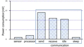
Figure 12 shows a typical sensor node energy consumption distribution. It is clear that wireless communication module is the main energy consumption unit. The radio energy dissipation model is defined as:
0 0 4 2 0 . . . . . . d d d d for for d k E k d k E k E mp elec fs elec Tx ≥ < ≤ ⎪⎩ ⎪ ⎨ ⎧ + + = ε
ε (15)
The amount of energy consumed for transmission ETx, of k-bit message over a distance d is given by equation (15). The energy expended in receiving a k-bit message is given by equation (16).
ERx=k.Eelec (16) Where Eelec is the amount of energy consumed in electronic circuits, εfs is the energy consumed in an amplifier when transmitting at a distance shorter than d0, and εmp is the energy consumed in an amplifier when transmitting at a distance greater than d0.
Figure 12. Distribution of energy consumption of sensor nodes
Every sensor node has the same initial energy (refer as Ei) and the same connection performance according to equation (9) at the start of the network to work. However, as time went on, the remainder energy of sensor node (refer as Eri) will be far different because the unbalance energy consumption. Thus the perception of the sensor nodes radius (rs) and the communication radius (rc) will be affected, and so do node's coverage and connectivity. As the network running time grows, the residual energy of sensor nodes reduces. When running time reaches a threshold (or the energy of the sensor node is less than a threshold), network coverage performance and connectivity will drop dramatically, as shown in Figure 13.
0 0.1 0.2 0.3 0.4 0.5 0.6 0.7 0.8 0.9 1 0 10 20 30 40 50 60 70 80 90 100
The ratio of remaining energy and primary energy of sensor nodes (Eir/Ei)
N e tw ork c ov erage ef fi c ient and c o m m un ic a ti on ef fi c ient (% )
Network coverage efficient Network communication efficient
Figure 13. Impact of the remaining energy of sensor nodes on network
coverage efficiency and network communication efficiency.
In order to accurately evaluate network connection performance, we design the Ns×7 network connection performance matrix which is described by equation (17). The matrix C[i][0] denotes the identifier of node si (i=0,Ns-1). C[i][1,2,3] denotes the X,Y,Z coordinates of si (i=0,Ns-1). C[i][4] denotes sis connection, C[i][5] the remainder energy and C[i][6] the network route path.
⎥ ⎥ ⎥ ⎥ ⎥ ⎦ ⎤ ⎢ ⎢ ⎢ ⎢ ⎢ ⎣ ⎡ s s s s s
s N N N N N
N
s X Y Z C E R
N R E C Z Y X R E C Z Y X # # # # # # # 2 2 2 2 2 2 1 1 1 1 1 1 2 1 identifier of node
X,Y,Z coordinate of node connection of node energy of node route path of node C=
(17)
D. Energy Prior Line Deployment Strategy
In order to avoid unbalanced energy consumption of WSN, we use the energy prior line deployment strategy of PSNs to prolong the life span of network. The deployment strategy is shown in figure 14.
Figure 14. Line PSNs deployment strategy
In figure 14, Ni denotes the number of PSNs in the i-th position of multi-hop data transmission route to ISSN. In order to keep the same ratios (refer as β) of energy consumption in each position to the total amount of energy in the position, we need to deploy more PSNs in the positions closer to ISSN, and less PSNs that are far from ISSN.βcan be determined by equation (18), where Ei-alldenotes the total energy consumption of PSNs in the i-th position. We can effectively prolong the life span of network by scheduling PSNs to switch between active state and sleeping state, so that each position has only one active PSN to sense and relay data packets to ISSN in the same time.
1 2
1 2
i n
all all i all n all
N N
N N
E E E E
β
− − − −
= = = =" = =" (18)
VI. CONCLUSION
node and the radius of a pipeline. We also present a complete algorithm description for the deployment model. We evaluated the presented 3D deployment model from the connectivity, coverage and energy consumption aspects. Empirical results showed that our algorithm is effective and efficient.
Although energy is an important issue in WSNs for pipeline systems, we only briefly discussed it in this work. In future, we plan to further investigate the energy and delay issues based on our three-dimensional sensing coverage model for pipeline systems
ACKNOWLEDGMENT
The authors are grateful to the anonymous referees for their valuable comments and suggestions. The research is supported by the PetroChina Innovation Foundation (Grant No. 2013D-5006-0605).
REFERENCES
[1] Hande Alemdar and Cem Ersoy, “Wireless sensor
networks for healthcare: A survey,” [J] Computer
Networks vol. 54 no.15, 2010, pp. 2688–2710.
[2] Luís M. L. Oliveira and Joel J. P. C. Rodrigues, “Wireless
Sensor Networks: a Survey on Environmental
Monitoring,” [J] Journal of communications, vol.6, no. 2,
April 2011, pp.143-151.
[3] J.Yick, B.Mukherjee, and D.Ghosal, “Wireless Sensor
Network Survey,” [J] Computer Networks: The International Journal of Computer and Telecommunications Networking, vol.52, no.12, 2008, pp.2292-2330.
[4] Guan Hua, Yan-Xiao Li and Xiao-Mei Yan “Research on
the Wireless Sensor Networks Applied in the Battlefield Situation Awareness System,” [C] International Conference, ECWAC 2011, Guangzhou, China, April 16-17, 2011.
[5] Yuanwei Jin and Ali Eydgahi, “Monitoring of Distributed
Pipeline Systems by Wireless Sensor Networks,”[C] Proceedings of the 2008 IAJC-IJME International Conference, 2008.
[6] J. Harada, S. Shioda and H. Saito, “Path Coverage
Prop-erties of Randomly Deployed Sensors with Finite Data- transmission Ranges,”[J] Computer Networks,vol.53, 2009, pp. 1014-1026.
[7] H. H. Zhang and J. C. Hou, “Maintaining Sensing
Cov-erage and Connectivity in Large Sensor Networks,” [J] Journal of Ad Hoc and Sensor Wireless Networks, vol. 1, no. 1-2, 2005, pp. 89-124.
[8] N. Heo and P. K. Varshney, “Energy-efficient deployment
of intelligent mobile sensor networks,”[J] IEEE Transactions on Systems, Man, and Cybernetics—Part A: Systems and Humans, vol. 35, no. 1, 2005, pp. 78–92.
[9] Peng-Jun Wan and Chih-Wei Yi, “Coverage by Randomly
Deployed Wireless Sensor Networks,”[J] IEEE Transactions on information theory, vol. 52, no. 6, 2006,pp.2658-2669.
[10] Gongbo Zhou, “The Reliability Supported Technologies of
Wireless Sensor Networks in Long-narrow Region,” [D]
The Doctor Dissertation of China University of Mining and Technology, June 2010.
[11] Huafeng Liu, “Research on the 3D Topology Organizing
and Clustering Algorithms in Sensor Networks,” [D] The
Doctor Dissertation of National University of Defense Technology, March, 2007.
[12] Jiang Peng, Liu Xiaoqing, “Coverage method based on
combined weighted clustering for 3D wireless sensor
networks,” [J] The Journal of Application Research of
Computers, Vol.28, No.5, May 2011, pp. 1824-1830.
[13] Zhang Baoli,Yu Fengqi, Zhang Zusheng, “An Energy
Efficient Three-Dimensional Coverage Control Algorithm
for Wireless Sensor Networks,” [J] The Journal of
Sensors and Actuators, Vol. 22, No.2, Feb. 2009, pp. 259-263.
[14] Li Caili, Feng Hailin, Hou Nan, “Energy-efficient coverage
algorithm in 3D wireless sensor network,” [J] The Journal
of Computer Application, Vol.30, No.7, July 2010, pp.1719-1724.
[15] Li li, Liu Yuan-an, “Sensor Deployment Algorithm for Wir
eless Underground Sensor Network” [J] The Journal of Ji
lin University (Information Science Edition), Vol.25, No.6, Nov. 2007, pp.587-592.
[16] Ammari H M, Das S K. “A Study of k-coverage and measu
res of connectivity in 3D wireless sensor networks,”[J]. IE EE Trans on Computers, vol.59, no.2, 2010, pp. 243-257.
[17] Pompili D, Melodia T and Akyildiz I F, “Three-dimension
al and two-dimensional deployment analysis for underwate r acoustic sensor networks,”[J] Elsevier Journal of Ad Hoc Networks, vol.7,no.4,2009,pp. 778-790.
[18] Wikipedia, “Pipeline transport,”[R] http://en.wikipedia.org
/wiki/Oil_pipeline#For_oil_or_natural_gas, 2013.2.
[19] Huaping Yu, “The Research of Hierarchical Data Fusion
based on Three-tiers Wireless Sensor Networks for Urban Real Time Traffic Information Monitoring,”[C] Proceedings of the fourth International Conference on
Genetic and Evolutionary Computing, Shenzhen China,
December 13-15, 2010:802~805.
[20] Hossaina, Biswaspk, Chakrabarti S. “Sensing models and
its impact on network coverage in wireless sensor network”[C]. Proceeding of the 2008 IEEE Region 10 Colloquium and the Third ICIIS, Kharagpur, 2008,pp 1-5.
[21] H.H.Zhang and J.C.Hou, “Maintaining Sensing Coverage
and Connectivity in Large Snesor Nwtworks,” [J] The
Journal of Ad Hoc and Sensor Wireless Networks, Vol.1, No.1-2, 2005, pp.89-124.
Huaping Yu received his B.S. and M.S.
degrees in Computer Engineering from the Yangtze University, Jingzhou, China, in 2001 and 2008, respectively.
He is currently a researcher in the oil and gas pipeline monitoring and wireless sensor network laboratory and pursuing his Ph.D. degree at the Institute of petroleum engineering Yangtze University, Wuhan, China. His current research interests include oil and gas field production safety monitoring and wireless sensor networks.
He is associate professor of College of Computer Science, Yangtze University. Recently, he has taken 9 research projects at all levels, and has more than 30 academic theses being published. Currently, he is the member of China computer federation.
Lan Huang received her Ph.D. in