Variance Reduction Techniques of Importance Sampling Monte Carlo Methods for Pricing Options

http://dx.doi.org/10.4236/jmf.2013.34045

Variance Reduction Techniques of Importance Sampling

Monte Carlo Methods for Pricing Options

*

Qiang Zhao1, Guo Liu1, Guiding Gu2

1_{School of Finance, Shanghai University of Finance and Economics, Shanghai, China} 2_{Department of Applied Mathematics, Shanghai University of Finance and Economics, Shanghai, China}

Email: [email protected]

Received July 10,2013; revised September 7, 2013; accepted September 18, 2013

Copyright © 2013 Qiang Zhao et al. This is an open access article distributed under the Creative Commons Attribution License, which permits unrestricted use, distribution, and reproduction in any medium, provided the original work is properly cited.

ABSTRACT

In this paper we discuss the importance sampling Monte Carlo methods for pricing options. The classical importance sampling method is used to eliminate the variance caused by the linear part of the logarithmic function of payoff. The variance caused by the quadratic part is reduced by stratified sampling. We eliminate both kinds of variances just by importance sampling. The corresponding space for the eigenvalues of the Hessian matrix of the logarithmic function of payoff is enlarged. Computational Simulation shows the high efficiency of the new method.

Keywords: Monte Carlo Method; Importance Sampling; Variance Reduction; Option Pricing

1. Introduction

Monte Carlo simulation is a numerical method based on the probability theory. Its application in finance becomes more and more popular as the demand for pricing and hedging of various complex financial derivatives, which play an important role in the field of investment, risk management and corporate governance. The advantage of Monte Carlo method is that its convergence rate is independent on the number of state variables. Monte Carlo simulation is often the only way available for the pricing of complex path-dependent options if the number of relevant underlying assets is greater than three. However, Monte Carlo simulation is constantly criticized for its slow convergence. Let be a random variable and we want to calculate

V

 

E V



 . We can generate independently and identically distributed samples

of V . Law of Large Numbers guarantees that

 

n₁ i i

V _

. .

n

1 1

n _i

i

V V

n

a s











and Central Limit Theorem guarantees that  asymp- totically falls in the confidence interval

2 2

,

n n

V Z V Z

n  n 

 



 

 

  

with probability , where  er of

1 is the standard devia- tion of V , n is the numb samples,  is the significance level and

2

Z_ is the quantile of standard

normal distribution under 2 

.

method is

It is clear that the convergence rate of Monte Carlo

1 2

O n_  _.

 

hence, in order to reduce the err by a factor of 10 one has to generate 100 times as mu as samples as well as computation time. For this reason, Monte Carlo simu-

or ch

lation needs to be run on large parallel computers with a high financial cost in terms of hardware and software developments. The computational demands of simulation have motivated substantial interest in the financial industry in demands for increased efficiency. Another way to improve the accuracy is to reduce the standard deviation . Motivated by this thought, several tech- niques to reduce the variance of the Monte Carlo simu- lation have been proposed, such as control variates, antithetic riables, importance sampling and stratifi- cation(see Boyle, Broadie and Glasserman [1], and Gla- sserman [2]. These techniques aim to reduce the variance per Monte Carlo observation so that a given level of

va

*_{This work is supported by Research Innovation Foundation of}

accuracy can be obtained with a smaller number of simulations. Control variates and antithetic variables are the most widely used variance reduction techniques, mainly because of the simplicity of their implementations, and the fact that they can be accommodated in an exist- ing Monte Carlo calculator with a small effort. Examples of successful implementations of control variates for pricing the derivatives include Hull and White [3], Kemna and Vorst [4], Turnbull and Wakeman [5], Ma and Xu [6].

Importance sampling has the capacity to exploit detailed knowledge about a model (often in the form of asymptotic approximations) to produce potential variance re

o

tantially by increasing the drift in simulation fo

ampling combined with stratified sampling to dr

ampling attempts to reduce variance by hich samples , consider the duction. Unfortunately, importance sampling technique

has not been widely used as other variance reduction techniques in pricing financial derivatives until recently. This is mainly because there is no general way to implement importance sampling. If the transformation of probability measure is chosen improperly, this method does not work. Importance sampling attempts to reduce variance by changing the probability measure from which paths are generated. Our goal is to obtain a more convenient representation of the expected value. The idea behind the importance sampling is to reduce the statis- tical uncertainty of Monte Carlo calculation by focusing on the most important region of the space from which the random samples are drawn. Such regions depend both on the random process simulated, and the structure of the security priced. Just as mentioned by Glasserman [2], an effective importance sampling density should weight more points to the region where the product of their probability and their payoff is large. For example, for a deep out-of-the-money call option, most of the time the payoff from simulation is 0, so simulating more paths with positive payoffs should reduce the variance in the estimation.

An early example of imp rtance sampling applied to security pricing is Reider [7], where the variance was reduced subs

r deep out-of-the-money European call options. Gla- sserman, Heidelberger and Shahabuddin [8] applied importance sampling to reduce substantial variance by combining stratification in the stochastic volatility model. Other recent work on importance sampling methods in finance has been done for Monte Carlo simulations driven by high-dimensional Gaussian vectors, such as Boyle, Broadie and Glasserman [1], Vázquez-Abad and Dufresne [9], Su and Fu [10], Arouna [11], Capriotti [12], Xu and Zhang [13]. In this framework, Importance Sampling is applied by modifying the drift term of the simulated process to construct a new measure in which more weight is given to important outcomes thereby increasing sampling efficiency. The different methods proposed in the literature mainly differ in the way where such a change of drift is found, and can be divided into

two families based on the strategy adopted. The first one is proposed by Glasserman, Heidelberge and Shaha- buddin in a remarkable paper [14] (GHS for short), relies on a deterministic optimization procedure which can be applied for a specific class of payoffs. Xu and Zhang [13] improve the optimization algorithm of the importance sampling by Newton Raphson algorithm based on direct simulation. The second one is the so-called adaptive Monte Carlo method, such as Vázquez-Abad and Du- fresne [9], Su and Fu [10], Arouna [11], that aims to determine the optimal drift through stochastic optimi- zation techniques that typically involve an iterative algo- rithm.

Most closely related to our work is Glasserman, Heidelberge and Shahabuddin [14], who applied impor- tance s

amatically reduce variance in derivative pricing. In this paper, we propose a new importance sampling method by modifying the drift term and the quadratic term of the simulated process simultaneously. In the previous literature, the variance for the linear part is eliminated by importance sampling and those for the quadratic part is reduced by stratification. However, we eliminate both kinds of variances just by importance sampling. The corresponding space for the eigenvalues of the Hessian matrix of the log function of payoff is enlarged. Illu- strations of the use of the method with European options and Asian options are given, which show the high effi- ciency of the method. The method proposed in the paper can be extended to the pricing of other financial deriva- ives directly.

2. Importance Sampling Method

Importance s

changing the probability measure from w are generated. To make this idea concrete problem of estimating

 

   

d ,

f

V E _G X _



G x f x x (1) where X is a random vector of with probability

density

n



f , and E_f

 

easure

denotes xpecta with density

the e function

tion under the original m f , G is a

functio from _n _{to  , gen lly denoting the}

payoffs financial derivatives. The ordinary Monte Carlo estimator is

n of

era

 

1

1

ˆ M _,

f i

i

V G X

M 





(2)

1, 2, , M

X X  X

with independent draws from f . Let

g be any other probability density on n satisfying

 

x > 0g x

 

> 0, (3) r all _xn_{. Then we can obtain b hanging mea-}

f

fo y c

   

f x

_{   }

d

_{   }

 

V 



G x g x xE G X

, can be interpreted as an expectation with respect t density

.

f X 

(4)

g

g x _ g X _

Thus V

o the g.

If X X1, 2, , XM are now independent draws from

g, the importance sampling estimator associated with g is

   

_{ }

1

1 M _.

i

g i

i i

f X Vˆ G X

M  g X





(5)

The weight

   

i i



 

i



f X g X w X

is the likelihood ratio evaluated at X_i. It follows from (1) and (4) that

ˆ ˆ _,

f f g g

E  _{ }V E  _{ }V V

and thus both Vˆf and Vˆg are un

. To compare variances with and without im

bi ed estimators of portance sampling it suffices to compare their second moments.

as V

With importance sampling we have

   

_{ }

   

_{ }

2

2 _.

g f

f X f X

E G X E G X

g X g X

_{ }  _{ }

_ _    

_{ }  _ _

 

(6)

Depending on the choice of g, this could be larger or smaller than the second mo  w importance sampling. Succe pling lies on t

ment

ssful

 

2

f

E G X importance sam

ithout he art of selecting an effective importance sampling density g.

From (2), the variance of Vˆf is

 



2

 

2



1 1

ˆ

Varf Vf Varf G X Ef G X V ,

M M

w

  _ _ _ _

 

here Varf

 

denotes the variance under the measure

with density function f . Similarly, from (5) and (6), the variance of Vˆg is

   



2 2



1

.

g ˆg Eg G X w X V

Var V

M

 

  

   

In particularly, if 

, a zero-variance estimate is thus obtained by choosing

0

V 

 

1

   

. g x G x f x

V We call this function as t

 (7) he optimal density function. This choice of density is precluded unless the estimated quantity is known from the outset. N

observation provides a useful insight: An effective im- V evertheless, this portance sampling density should weight points ac- cording to the product of their probability and payoff.

Generally, the key of importance sampling lies to find g satisfying (3) to solve the following optimal problem,

   

_{ }

2

ming f .

f X

E G X

g X

 

 

 

 

Unfortunately, there is no general way to find the (8)

optimal g for an ordinary function f . So, we find the relatively optimal

turn to g to m

small as possible.

Im

i

a

dea of GHS. Consider the ake the variance as

3. New

portance Sampling S mulation

In this section, we propose new importance sampling simulation following the i

problem of estimating the expectation of the payoff

 

n

   

d ,

f _R

V E _G X _



G x f x x

where X is a n -dimensional vector of standard normal variable with probability density

   

1₂





T

2 _{1 2}

n

when choosing the new probability functio

2π ne x xT , , , , .

f x    x x x  x

n, the previous literature featuring GHS has only taken drift into consideration. They choose drift  satisfying

   

_{ }

2

min f ,

f X E G X

g X





 

 

 

  (9)

where

   

_{2π 2e} 12   T

n _{x x}

g x  

  



 .

Based term into

on GHS’s idea, we take both drift and variance consideration. If the covariance matrix  is positive definite, we can choose

   

2π 2 12e 12  1 ,

T

n x x

g x  



   

 

  (10)

thus, we obtain by changing measure

   

_{   }

   

_{ }

   

d

,

n R

g g

f x

V G x g x x

g x

E G X E G X w X

g X



 _{ } _ _

 

 



(11)

where the likelihood ratio is f X

 

 

1_2e 12 12  1 _.

T T

x x x x

w x  



    

 

Note that the covariance ma there exists a nonsingular

trix is positive definite, ensional matrix



-dim

n A

satisfying _{ AA}T_.

If



0, n



Z N I ,

and

then

Denote



,



X N   .

 

log



 



F x  G x ,

where

0 It follows that

 





, n:

xD D xR G x  .

   



 













 



 

 











1 2exp E F 1 1 2 1 1 exp 2 2 exp 1 1 . 2 2 f f T T T f

T T T

n

V E X w X

E G AZ w AZ

AZ

g G

AZ AZ AZ AZ

E F AZ AZ

Z A A I Z

            _   _     _     _              _  (12) Suppose that  _   F -ord

is twice continuously differentiable on D, a second er Taylor expansion formula shows





 

 

 

2

  

 

2 2

T

1

T

F AZ F F AZ

AZ F  AZ o Z

  

     

By (12) and (13), we have

(13)

 



 



 



 



 

 

1 2 2 1 1 exp 2 . 2 T T f n

V E F F

AZ o Z

         _ _             2 1 T

AZ F  I

  

AZ

 

(14) We can choose ˆ and satisfying ˆ

 

ˆ ˆ

F  

  (15) and

(16) where we assume that all the eigenvalues of the Hessian

ix

 



₂



1 ˆ _{I F ˆ}  _,    

matr F

 

ˆ of Rogers and Talay

are less than . (Following the analysis [15], th ondition

most of options including Asian option 1

e c is satisfied for , barrier option and various path-dependent options with stochastic vola- tility.)

(15) can be solved using iteration method in GHS. Then, ˆ is easily obtained by direct substitution of ˆ . So the linear and quadratic part of the function F is

may be

removed. Our choice of drift vector and variance matrix

viewed as eliminating the variance contribution due to the linear and the quadratic part of F . We

conside the new density function

   

r

  1 

1 1 _{ˆ ˆ ˆ} 2 2

2 ˆ

2π e

T

n _{x x}

g x  



    



  (17) as a proper measure transformation. Finally, the new estimator with smaller variance can be obtained b

In GHS, the variance caused by

y tic part of

(5). the quadra

F is reduced by use of stratification whi

relatively complicated numerical calculation. Meanwhile, ch needs the efficiency of the stratification demands that all the eigenvalues of the Hessian matrix of F at the value ˆ

are less than 1

2. Obviously, the new method can be applied to more types of financial derivatives.

4. Numerical Simulation

In this section, we illustrate the results developed in the previous sections. We use two examples in

compare our method with GHS method to rew we the the price of un rlying

hich veal de efficiency of the new method.

In the Black-Scholes model, asset S t

 

obeys

 

 

 

 

dS t rS t dtS t dW t , (18) where r is the risk free rate ,  is the volatility and

 

t is a standard Brownian motion.

Supp that

W

ose

 

0, T is the period of t e option

and is the number of observations, valid h

n

 

ti i1

n

 are the

observa on dates and S t

 

i s the price of the

ing asset at the ith observation date.

ti i

underly

asse

The underlying t can be simulated by

 

 

_exp 1 2





S t S t _{1 }_r  _ t t ₁  t ₁X _

2 1, 2, , ,

i i i i i i i

i n          t  (19) where





T

 

1, 2, , n 0,

X  X X  X N I .

For simplicity, we set

1 , 1, 2, ,

i i

t t_   t T n i  n.

Experiment 1: Consider European call option under the Black-Scholes model. The discounted pa ff function yo is

 

e rTmax



 

,0



G X   S T K .

We set S

 

0 50, 0.05, 1.0, 16r T  n and use

1,000,000

M  paths to estimate the variance reduction ratio between Varf G X

 

 and VargG X

   

w X .

Numerical results in Table 1 show est ated prices and variance ratios, relative to ordinary Monte Carlo m g importance sampling with GH

and the new m

f the proced r this problem, es- eduction ra

im

ethod, usin S method

ethod respectively, which confirm the effectiveness o ure fo

pecially for in-the-money options. Variance r

tio is the variance per replication using standard Monte Carlo method divided by the variance per replication using the above two methods. The large ratio, the great the improvement.

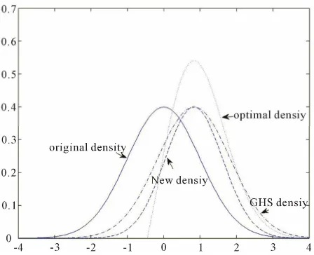
In Figure 1, the optimal density denotes the density represented by (7). The GHS density figure can be obtained through translating the original density figure right by . After modifying the quadratic term, we can change the shape of the GHS density figure and get the new density figure. Obviously, the new density figure is closer

e

to the optimal one than the GHS density figure, thus achieving greater variance reduction.

Experiment 2: As a typical test case treated in recent papers, w will consider arithmetic Asian call option. The discounted payoff function is

 

 

1 1

e rTmax n ,0 .

i i

G X S t K

n





 

 _  _







We set S

 

0 50, 0.05, 1.0, 16r T  n and use

1000000

M  paths to estimate the variance reduction

ratio between Varf G X

 

 and 

   

w X .

.

Varg G X

rical results are illustrated in Tables 2-6



These tables above show the simulation results for different volatilities and strike prices. Firstly, GHS m es larger variance ratios when th

deeper out o

deep out-o y Call option, mos . By ch

The nume

ethod achiev e option is f money, which coincides with results in Reider [7]. For a f-mone t paths with zero payoff are sampled in simulation

[image:5.595.310.534.86.268.2]

anging the drift of sampling density, a large part of zero-payoff paths are replaced by positive-payoff paths. Hence, simulating more samples with positive payoff reduces the variance. The effect of variance reduction by changing the drift will be strengthened or weakened by changing the form of the sampling density figure.

Table 1. Estimated variance reduction ratios for European call option.

Parameters IS (GHS method) IS (new method)

 K Price VarRatio Price VarRatio

0.1 30 21.463 103.3 21.463 931.2

45 7.317 8.2 7.316 15.9

50 3.404 7.2 3.405 12.1

0.

55 1.087 11.2 1.088 12.5

3 30 21.602 14.9 21.601 30.0

45 9.869 9.5 9.855 15.9

50 7.118 10.3 7.121 15.8

55 5.010 11.8 5.014 5.9

[image:5.595.307.540.336.408.2]

Figure 1. Sampling probability density function for Euro- pean call option with  0.1,K50.

Table 2. Estimated variance reduction ratios for arithme- tic Asian call option with  0.05.

Parameters IS (GHS method) IS (new method)

K Price VarRatio Price VarRatio

45 6.042 39.8 6.042 931.2

7 13 0.007 35.9

50 1.437 6.4 1.438 11.5

[image:5.595.308.540.448.520.2]

55 0.00 8.1

Table 3. Estimated va r ra or -

tic Asian w

riance eduction tios f arithme call option ith  0.1.

Parameters IS (GHS method) IS (new method)

K Price VarRatio Price arRatiV o

45 6.055 10.8 6.055 24.5

2 0.202 13.3

50 1.919 7.0 1.919 11.9

[image:5.595.309.539.560.631.2]

55 0.202 21.

Table 4. Estimated va r ra or -

tic Asian w

riance eduction tios f arithme call option ith  0.2.

Parameters IS (GHS method) IS (new method)

K Price VarRatio Price arRatiV o

45 6.418 7.7 6.419 14.5

50 3.028 8.2 3.028 13.4

[image:5.595.56.290.596.734.2]

55 1.106 13.0 1.106 14.0

Table 5. Estimated v e r or -

tic Asian w

arianc reduction atios f arithme call option ith  0.3.

Parameters IS (GHS method) IS (new method)

K Price VarRatio Price arRatiV o

45 7.150 8.3 7.151 15.0

50 4.169 9.2 4.169 14.9

[image:5.595.309.541.672.736.2]

Tabl ted v n ra

e-tic Asian w

http://dx.doi.org/10.2307/2331065 e 6. Estima ariance reductio tios for arithm

call option ith 0.5. _{[4] A. G. Kemna and A. C. F. Vorst, “A Pricing Method for} Options Based on Average Asset Values,” Journal of Banking & Finance, Vol. 14, No. 1, 1990, pp. 113-129. http://dx.doi.org/10.1016/0378-4266

Parameters IS (GHS method) IS (new method)

K Price VarRatio Price arRatiV o (90)90039-5

-

45 8.996 10.6 8.996 18.6

50 6.459 11.

[5] S. Turnbull and L. Wakeman, “A Quick Algorithm for Pricing European Average Options,” Journal of Financial and Quantitative Analysis, Vol. 26, No. 3, 1991, pp. 377

389. http://dx.doi.org/10.2307/2331213 6 6.457 18.7

55 4.455 13.5 4.543 18.9

Secon , for an in o n ew achieves larger vari atio n th S m d With th ecrease o

[6] J. Ma and C. Xu, “An Efficient Control Variate Method for Pricing Variance Derivatives under Stochastic Vola- tility and Jump Diffusion Models,” Journal of Computa- tional and Applied Mathematics, Vol. 2

dly -the-m ney optio , the n method . ance r s tha e GH etho

e d f  , the rior com b- 35, No. 1, 2010,

vious. T is beca e fact that path ositive payoff are sam when simulating an in-the-

supe ity be es o

pp. 108-119. http://dx.doi.org/10.1016/j.cam.2010.05.017 [7] R. Reider, “An Efficient Monte Carlo Technique for

Pricing Options,” Working Paper, Wharton School, Uni- versity of Pennsylvania, Philadelphia, 1993.

[8] P. Glasserman, P. Heidelberger and P. Shahabuddin, “Im-

his use th most s with p

m

pled

oney option makes it ineffective just by changing the drift. When the volatility  gets smaller, the under- lying asset changes mor slow so that most payoffs are positive. This leads to the GHS method in vain and makes the new method effective.

Thirdly, for an out-of-the-money option, the GHS method performs better than the new method especially when the volatility

e

 is small. In this case, by chang- ing the drift, most paths with zero payoff are replaced by nonzero-payoff paths, leaves no room for more variance re

portance Sampling in the Heath-Jarrow-Morton Frame- work,” Journal of Derivatives, Vol. 7, No. 1, 1999, pp.

32-50. http://dx.doi.org/10.3905/jod.1999.319109 [9] F. J. Vázquez-Abad and D. Dufresne, “Accelerated Simu-

lation for Pricing Asian Options,” Proceedings of 1998 Winter Simulation Conference, Washington DC, 13-16

December 1998, pp. 1493-1500.

http://dx.doi.org/10.1109/WSC.1998.746020

[10] Y. Su and M. C. Fu, “Simulation in Financial Engineering: Importance Sampling in Derivative Securities Pricing,”

Proceedings of the 32nd Confer

tion, Society for Computer Simulation Interna duction by changing the form of the sampling density

function.

5. Concluding Remarks

In this paper, a new importance sampling Monte Carlo method for pricing options is proposed. Unlike the classical i

ence on Winter Simula- tional, 2000,

Least-squares Importance Sampling for

762435 pp. 587-596.

[11] B. Arouna, “Robbins-Monro Algorithms and Variance Reduction in Finance,” Journal of Computational Fi- nance, Vol. 7, No. 2, 2004, pp. 35-62.

[12] L. Capriotti, “

mportance sampling procedure, both kinds of art and the quadratic part ayoff are eliminated

ntrol, Vol. 21, No. 8, 1997, pp.1267-1321. http://dx.doi.org/10.1016/S0165-1889(97)00028-6 variance caused by the linear p

of the logarithmic function of p . The Monte Carlo Security Pricing,” Quantitative Finance, Vol.

8, No. 5, 2008, pp. 485-497.

http://dx.doi.org/10.1080/14697680701 corresponding space for the eigenvalues of the Hessian

matrix of the logarithmic function of payoff is enlarged. Computational Simulation shows the high efficiency of the new method.

REFERENCES

[1] P. Boyle, M. Broadie and P. Glasserman, “Monte Carlo Methods for Security Pricing,” Journal of Economic Dy- namic and Co

, 2011.

habuddin,

pp. 117-152. [13] C. Xu and L. Zhang, “On Optimal Drift Vector and Im-

portance Sampling for Pricing Options Based on Direct Simulations,” Working Paper

[14] P. Glasserman, P. Heidelberger and P. Sha

“Asymptotically Optimal Importance Sampling and Stra- tification for Pricing Path-Dependent Options,” Mathe- matical Finance, Vol. 9, No. 2, 1999,

http://dx.doi.org/10.1111/1467-9965.00065

[15] L. C. G. Rogers and D. Talay, “Numerical Methods in Finance,” Cambridge University Press, Cambridge, 1997. http://dx.doi.org/10.1017/CBO9781139173056

[2] P. Glasserman s in Financial En-gineering,” Springer-Verlag

, “Monte Carlo Method , New York, 2004.