ISSN (e): 2250-3021, ISSN (p): 2278-8719
Vol. 05, Issue 04 (April. 2015), ||V2|| PP 18-27
Numerical Study on MHD Flow And Heat Transfer With The
Effect Of Microrotational Parameter In The Porous Medium
R.K.Mondal
**B. M. Jewel Rana, R. Ahmed
*Mathematics Discipline Khulna University, Bangladesh. Mathematics Discipline Khulna University, Bangladesh. Mathematics Discipline Khulna University, Bangladesh.
Abstract: The numerical studies are performed to examine the Micropolar fluid flow past an infinite vertical plate. Finite difference technique is used as a tool for the numerical approach. The micropolar fluid behaviour on two- dimensional unsteady flow have been considered and its nonsimilar solution have been obtained. Nonsimilar equations of the corresponding momentum, angular momentum and continuity equations are derived by employing the usual transformation. The dimensionless nonsimilar equations for momentum, angular momentum and continuity equations are solved numerically by finite difference technique. The effects on the velocity, micro rotation and the spin gradient viscosity of the various important parameters entering into the problem separately are discussed with the help of graphs.
Keywords: Micropolar fluid, unsteady, Explicit finite difference method, Porous medium.
I.
INTRODUCTION
Because of the increasing importance of materials flow in industrial processing and elsewhere and the fact shear behavior cannot be characterized by Newtonian relationships, a new stage in the evaluation of fluid dynamic theory is in the progress. Eringen(1966) proposed a theory of molecular fluids taking into account the internal characteristics of the subtractive particles, which are allowed to undergo rotation. Physically, the micropolar fluid can consists of a suspension of small, rigid cylindrical elements such as large dumbbell-shaped molecules. The theory of micropolar fluids is generating a very much increased interest and many classical flows are being re-examined to determine the effects of the fluid microstructure. The concept of micropolar fluid deals with a class of fluids which exhibit certain microscopic effects arising from the local structure and micromotions of the fluids elements. These fluid contain dilute suspension of rigid macromolecules with individual motions that support stress and body moments and are influenced by spin inertia. Micropolar fluids are those which contain micro-constituents that can undergo rotation, the presence of which can affect the hydrodynamics of the flow so that it can be distinctly non-Newtonian. It has many practical applications, for example analyzing the behavior of exotic lubricants, the flow of colloidal suspensions, polymetric fluids, liquid crystals, additive suspensions, human and animal blood, turbulent shear flow and so forth.
Peddision and McNitt(1970) derived boundary layer theory for micropolar fluid which is important in a number of technical process and applied this equations to the problems of steady stagnation point flow, steady flow past a semi-infinite flat plate. [1] Eringen (1972) developed the theory of thermo micropolar fluids by extending the theory of micropolar fluids.The above mentioned work they have extended the work of El-Arabawy (2003) to a MHD flow taking into account the effect of free convection and micro rotation inertia term which has been neglected by El-Arabawy (2003) [3] . However, most of the previous works assume that the plate is at rest. Free-convection flow with thermal radiation and mass transfer past a moving vertical porous plate have analyzed by Makinde, O. D [9]. Unsteady MHD free convection flow of a compressible fluid past a moving vertical plate in the presence of radioactive heat transfer have been discussed by Mbeledogu, I. U, Amakiri, A.R.C and Ogulu, A, [10]. Numerical Study on MHD free convection and mass transfer flow past a vertical flat plate has been discussed by S. F. Ahmmed [11].
In our present work, we have studied about numerical study on Numerical study on micropolar fluid flow through vertical plate.The governing equations for the unsteady case are also studied. Then these governing equations are transformed into dimensionless momentum, energy and concentration equations are solved numerically by using explicit finite difference technique with the help of a computer programming language Compaq visual FORTRAN 6.6. The obtained results of this problem have been discussed for the different values of well-known parameters with different time steps. The tecplot is used to draw graph of the flow.
II.
MATHEMATICAL FORMULATION
-axis respectively,
0
u
v
x
y
(1)' 2 2
0 2
(
)
uB
u
u
u
u
u
v
g
T
T
t
x
y
y
y
(2)2
2
u
u
v
t
x
y
j y
j y
(3)2
2
p
T
T
T
k
T
u
v
t
x
y
C
y
(4)The boundary conditions for the problem are:
at
0;
u
0;
v
0;
0;
T
0
every whereat
0
0;
0;
0;
0
0
0;
0;
1;
1
0
0;
0;
0;
0
u
v
T
at x
u
v
T
at y
u
v
T
at y
(5)It is required to make the given equations dimensionless. For this intention we introduce the following dimensionless quantities
2 2
0 0 0 0
0 0
,
,
,
,
,
,
wU
U
u
v
U
U
X
x
Y
y
U
V
t
T
T T
T
U
U
Finally, we obtain
0
U
V
X
Y
(6)
2 ' 022
1
rUB
U
U
V
U
U
V
G T
X
Y
Y
Y
(7)2
2
U
U
V
X
Y
Y
Y
(8)2
2
1
r
T
T
T
T
U
V
X
Y
P
Y
(9)The corresponding boundary conditions for the problem are reduced in the following from
at,
0,
U
0,
V
O
,
0,
T
0
everywhere0,
0,
0,
0
0
0
0,
0,
1,
1
0
0,
0,
0,
0
U
V
T
at X
U
V
T
at Y
U
V
T
at Y
(10)III.
NUMERICAL SOLUTIONS
Many physical phenomena in applied science and engineering when formulated into mathematical models fall into a category of systems known as non-linear coupled partial differential equations. Most of these problems can be formulated as second order partial differential equations. A system of non-linear coupled partial differential equations with the boundary conditions is very difficult to solve analytically. For obtaining the
solution of such problems we adopt advanced numerical methods. The governing equations of our problem contain a system of partial differential equations which are transformed by usual transformations into a non-dimensional system of non-linear coupled partial differential equations with initial and boundary conditions. Hence the solution of the problem would be based on advanced numerical methods. The finite difference Method will be used for solving our obtained non-similar coupled partial differential equations.
From the concept of the above discussion, for simplicity the explicit finite difference method has been used to solve from equations (6) to (9) subject to the conditions given by (10).To obtain the difference equations the region of the flow is divided into a grid or mesh of lines parallel to X and Y axis is taken along the plate and Y -axis is normal to the plate.
Here the plate of height
X
max( 20)
i.e.X
varies from 0 to 20 and regardY
max( 50)
as corresponding toY
i.e. Y varies from 0 to 50. There are m=100 and n=200 grid spacing in the X and Y directions respectively.It is assumed that ΔX and ΔY are constant mesh sizes along X and Y directions respectively and taken as follows,
0.20 0
20
X
x
0.25 0
50
Y
x
with the smaller time-step, Δt=0.005.
Now using the finite difference method we convert our governing equations in the following form
, 1, , , 1
0
i j i j i j i j
U
U
V
V
X
Y
(11)
'
, , , 1, , 1 , , 1 , , 1
, , 2
, 1 ,
, 2
1
( )
i j i j i j i j i j i j i j i j i j
i j i j
i j i j
r i j
U U U U U U U U U
U V
X Y Y
G T MU
Y
(12) ', , 1, , 1 , , 1 , , 1
,
, , 2
, 1 ,
2
(
)
i j i j i j i j i j i j i j i j
i j
i j i j
i j i j
U
V
X
Y
Y
U
U
Y
(13) ', , 1, , 1 , , 1 , , 1
,
, , 2
1
2
(
)
i j i j i j i j i j i j i j i j
i j
i j i j
r
T
T
T
T
T
T
T
T
T
U
V
X
Y
P
Y
(14)And the initial and boundary conditions with the finite difference scheme are
0 0 0 0 , , , , 0, 0, 0, 0, ,0 ,0 ,0 ,0 , , , ,
0,
0,
0,
0
0,
0,
0,
0
0,
0,
1,
1
0,
0,
0,
0
i j i j
i j i j
n n n n j j j j n n n n i i i i n n n n
i L i L
i L i L
U
V
T
U
V
T
U
V
T
U
V
T
(15)
Here the subscripts
i
andj
designate the grid points withx
andy
coordinates respectively.IV.
RESULTS AND DISCUSSION
The effects of unsteady micropolar fluid behavior on a heated plate have been investigated using the finite difference technique. To study the physical situation of this problem, we have computed the numerical values by finite difference technique of velocity, micrirotation and temperature effect at the plate. It can be seen that the solutions are affected by the parameters namely, Microrotation parameter (∆), Spin gradient viscosity parameter (𝛬), Magnetic parameter (M), the vortex viscosity parameter (), Grashof Number (𝐺𝑟) and Prandtl
velocity U, microrotation Γ′and temperature 𝑇′ for different values of Microrotation parameter (∆), Spin gradient viscosity parameter (𝛬), the vortex viscosity parameter (), Grashof Number (𝐺𝑟) Prandtl number (𝑃𝑟). For these computations the results have been calculated and presented graphically by dimensionless time = 10 up to = 80. The results of the computations show little changes for = 10to = 60. But while arising at = 70 and 80 the results remain approximately same but microrotation. Thus the solution for
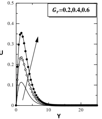
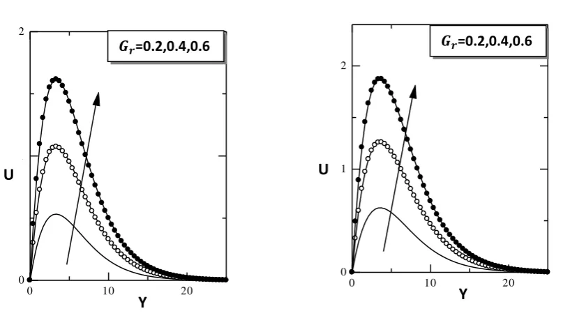
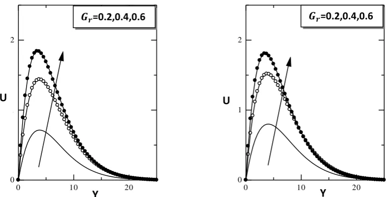
= 80 are become steady-state. Moreover, the steady state solutions for transient values of U, Γ′ and 𝑇′ are shown in figures 1- 24), for time = 10, 20, 30, 40, 50, 60, 70, 80 respectively. The values of Microrotation parameter (∆ = 0.01) is fixed. Whereas, figures (1-8) show the velocity profile for different values of Grashof Number (𝐺𝑟 = 0.2,0.4,0.6) at time = 10, 20, 30,40, 50, 60, 70, 80 respectively. From this figures it is
observed that the velocity profile increase with the increase of Grashof Number(𝐺𝑟), and the velocity profiles
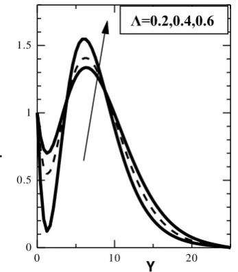
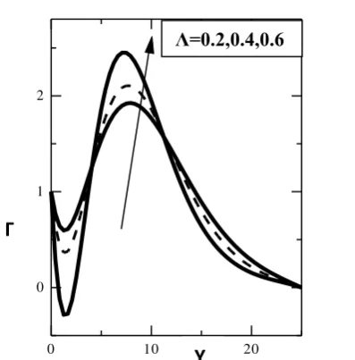
are going upward direction. While arising at = 70 and 80 the solutions become steady-state. Other important effects of microrotations are shown in figures (9-16) for different values of Spin gradient viscosity parameter
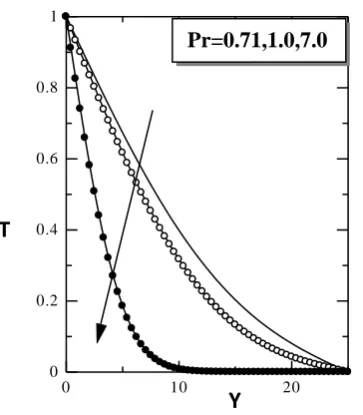
(𝛬) at time = 10, 20, 30, 40, 50,60, 70, 80 respectively. It is seen from this figures that the microrotaion increases with the increase of Spin gradient viscosity parameter (𝛬) and is going to the upward direction from the horizontal wall with the increase of time. While arising at = 70 and 80 the results also increasing with time. Other effects of temperature are shown in figures (17-24) for different values of Prandtl number (𝑃𝑟 = 0.71, 1.0, 7.0) at time = 10, 20, 30, 40, 50, 60, 70, 80 respectively.
One the other hand, at salt water the Prandtl number is(𝑃𝑟 = 1.0 ). It is seen from this figures that the
temperature distribution is decreases with the increase of Prandtl number and the flow pattern is directed to the outer wall with the increase of time. While arising at = 70 and 80 the flow becomes steady state
Fig. 1: Velocity Profile for different values of
Grashoff Number (
𝐺
𝑟) and
∆
= 0.01, M = 0.02 at
time
𝜏
= 10
Fig. 2: Velocity Profile for different values of
Grashoff Number (
𝐺
𝑟) and
∆
= 0.01, M = 0.02 at
time
𝜏
= 20
0 10 20
0 0.1 0.2 0.3 0.4 0.5
0 10 20
0 0.2 0.4 0.6 0.8
𝑮
𝒓=0.2,0.4,0.6
𝑮
𝒓=0.2,0.4,0.6
U
U
Fig. 3: Velocity Profile for different values of
Grashoff Number (
𝐺
𝑟) and
∆
= 0.01, M = 0.02 at
time
𝜏
= 30
Fig. 4: Velocity Profile for different values of
Grashoff Number (
𝐺
𝑟) and
∆
= 0.01, M = 0.02 at
time
𝜏
= 40
Fig. 5: Velocity Profile for different values of
Grashoff Number (
𝐺
𝑟) and
∆
= 0.01,M = 0.02 at
time
𝜏
= 50
Fig. 6: Velocity Profile for different values of
Grashoff Number (
𝐺
𝑟) and
∆
= 0.01, M = 0.02
at time
𝜏
= 60
0 10 20
0 0.5 1
0 10 20
0 0.5 1 1.5
0 10 20
0 1 2
0 10 20
0 1 2
𝑮
𝒓=0.2,0.4,0.6
𝑮
𝒓=0.2,0.4,0.6
𝑮
𝒓=0.2,0.4,0.6
𝑮
𝒓=0.2,0.4,0.6
U
U
U
U
Y
Y
Fig. 7: Velocity Profile for different values of
Grashoff Number (
𝐺
𝑟) and
∆
= 0.01, M = 0.02 at
time
𝜏
= 70
Fig. 8: Velocity Profile for different values of
Grashoff Number (
𝐺
𝑟) and
∆
= 0.01, M = 0.02
at time
𝜏
=80
Fig. 9: Microrotation Profile for different values
of Spin Gradient viscosity parameter(Λ) and ∆ =
0.01, M = 0.02 at time
𝜏
= 10
Fig. 10: Microrotation Profile for different
values of Spin Gradient viscosity parameter(Λ)
and ∆ = 0.01, M = 0.02 at time
𝜏
= 20
0 10 20
0 1 2
0 10 20
0 1 2
0 10 20
0 0.2 0.4 0.6 0.8 1
0 10 20
0 0.2 0.4 0.6 0.8 1
𝑮
𝒓=0.2,0.4,0.6
𝑮
𝒓=0.2,0.4,0.6
Λ=0.2,0.4,0.6
Λ=0.2,0.4,0.6
U
U
Y
Y
Г
Г
Fig. 11: Microrotation Profile for different values
of Spin Gradient viscosity parameter(Λ) and ∆ =
0.01, M = 0.02 at time
𝜏
= 30
Fig. 12: Microrotation Profile for different values
of Spin Gradient viscosity parameter(Λ) and ∆ =
0.01, M = 0.02 at time
𝜏
= 40
Fig. 13: Microrotation Profile for different values
of Spin Gradient viscosity parameter(Λ) and ∆ =
0.01, M = 0.02 at time
𝜏
= 50
Fig. 14: Microrotation Profile for different
values of Spin Gradient viscosity parameter(Λ)
and ∆ = 0.01, M = 0.02 at time
𝜏
= 60
0 10 20
0 0.2 0.4 0.6 0.8 1
0 10 20
0 0.5 1
0 10 20
0 0.5 1 1.5
0 10 20
0 1 2
Λ=0.2,0.4,0.6
Λ=0.2,0.4,0.6
Λ=0.2,0.4,0.6
Λ=0.2,0.4,0.6
Г
Г
Г
Г
Y
Y
Fig. 15: Microrotation Profile for different values
of Spin Gradient viscosity parameter(Λ) and ∆ =
0.01, M = 0.02 at time
𝜏
= 70
Fig. 16: Microrotation Profile for different values
of Spin Gradient viscosity parameter(Λ) and ∆ =
0.01, M = 0.02 at time
𝜏
= 80
Fig. 17: Temperature Profile for different values
of Prandtl Number (
𝑃
𝑟) and M = 0.02 at time
𝜏
=
10
Fig. 18: Temperature Profile for different values
of Prandtl Number (
𝑃
𝑟) and M = 0.02 at time
𝜏
=
20
0 10 20
0 1 2
0 10 20
0 1 2 3
0 10 20
0 0.2 0.4 0.6 0.8 1
0 10 20
0 0.2 0.4 0.6 0.8 1
Λ=0.2,0.4,0.6
Λ=0.2,0.4,0.6
Pr=0.71,1.0,7.0
Pr=0.71,1.0,7.0
Г
Г
T
T
Y
Y
Fig. 19: Temperature Profile for different values
of Prandtl Number (
𝑃
𝑟) and M = 0.02 at time
𝜏
=
30
Fig. 20: Temperature Profile for different values
of Prandtl Number (
𝑃
𝑟) and M = 0.02 at time
𝜏
=
40
Fig. 21: Temperature Profile for different values
of Prandtl Number (
𝑃
𝑟) and M = 0.02 at time
𝜏
=
50
Fig.22: Temperature Profile for different values
of Prandtl Number (
𝑃
𝑟) and M = 0.02 at time
𝜏
=
60
0 10 20
0 0.2 0.4 0.6 0.8 1
0 10 20
0 0.2 0.4 0.6 0.8 1
0 10 20
0 0.2 0.4 0.6 0.8 1
0 10 20
0 0.2 0.4 0.6 0.8 1
Pr=0.71,1.0,7.0
Pr=0.71,1.0,7.0
Pr=0.71,1.0,7.0
Pr=0.71,1.0,7.0
T
T
T
T
Y
Y
Fig. 23: Temperature Profile for different values
of Prandtl Number (
𝑃
𝑟) and M = 0.02 at time
𝜏
=
70
Fig. 24: Temperature Profile for different values
of Prandtl Number (
𝑃
𝑟) and M = 0.02 at time
𝜏
=
80
REFERENCES
[1] Eringen, A.C., (1966), Journal of Mathematical Mechanics,16,1
[2] Eringen, A.C., (1972), Journal of Mathematical Analysis Applied,38,480
[3] El-Arabawy,H.A.M.,(2003)., International Journal of Heat and Mass Transfer,46,1471 [4] Peddiesen,j., and McNitt,R.P., (1970),Recent Advanced Engineering Science,5,405 [5] Callahan,G.D. and Marner,W.J.(1976).Int.J.Heat Mass Transfer,19,165
[6] Soundalgekar and Ganesan(1980).,International Journal of Engineering andScience,18,287
[7] P.Chandran, N.C.Sacheti and A.K.Singh, “Unsteady free convection flow with heat flux and accelerated motion.” J. Phys. Soc. Japan 67,124-129, 1998.
[8] V. M. Soundalgekar, B. S. Jaisawal, A. G. Uplekar and H. S. Takhar, “The transient free convection flow of a viscous dissipative fluid past a semi-infinite vertical plate.” J. Appl. Mech. Engng.4, 203-218, 1999. [9] O. D Makinde “Free-convection flow with thermal radiation and mass transfer past a moving vertical
porous plate”, Int. Comm. Heat Mass Transfer, 32, pp. 1411– 1419, 2005
[10] Mbeledogu, I. U, Amakiri, A.R.C and Ogulu “Unsteady MHD free convection flow of a compressible fluid past a moving vertical plate in the presence of radioactive heat transfer”, Int. J. of Heat and Mass Transfer, 50, pp. 1668– 1674, 2007.
[11] S. F. Ahmmed, S. Mondal and A. Ray.” Numerical studies on MHD free convection and mass transfer flow past a vertical flat plate”. IOSR Journal of Engineering (IOSRJEN). ISSN 2250-3021, vol. 3, Issue 5, pp 41-47, May. 2013.
0 10 20
0 0.2 0.4 0.6 0.8 1
0 10 20
0 0.2 0.4 0.6 0.8 1