ISSN (e): 2250-3021, ISSN (p): 2278-8719 Vol. 05, Issue 03 (March. 2015), ||V3|| PP 01-07
wavelet collocation method for solving integro-differential
equation.
Asmaa Abdalelah Abdalrehman
University of Technology Applied Science Department
Abstract: - Wavelet collocation method for numerical solution nth order Volterra integro diferential equations (VIDE) by expanding the unknown functions, as series in terms of chebyshev wavelets second kind with unknown coefficients. The aim of this paper is to state and prove the uniform convergence theorem and accuracy estimation for series above. Finally, some illustrative examples are given to demonstrate the validity and applicability of the proposed method.
Keywords: chebyshev wavelets second kind; integro-differential equation; operational matrix of integrations; uniform convergence; accuracy estimation.
I. INTRODUCTION
Basic wavelet theory is a natural topic. By name, wavelets date back only to the 1980s. on the boundary between mathematics and engineering, wavelet theory shows students that mathematics research is still thriving, with important applications in areas such as image compression and the numerical solution of differential equations [1], integral equation [2],and integro differential equations [3,8]. The author believes that the essentials of wavelet theory are sufficiently elementary to be taught successfully to advanced undergraduates [4].
Orthgonal functions and polynomials series have received considerable attention in dealing with various problems wavelets permit the accurate representation of a functions and operators. Special attention has been given to application of the Legendre wavelets [5], Harr wavelets [6] and Sine-Cosine wavelets [7]. The solution of integro-differential equations have a major role in the fields of science and ingineering when aphysical system is modeled under the differential sense, it finally gives a differential equation, an integral equation or an integro-differential equations mostly appear in the last equation [8].
In this paper the operational matrix of integration for Hermite wavelets is derived and used it for obtaining approximate solution of the following nth order VIDE.
u(n)(x)=g(x)+ 𝑘 𝑥, 𝑡 𝑢0𝑥 (𝑠) 𝑡 𝑑𝑡 (1) where 𝑛 ≥ 𝑠 k(x,t) and g(x) are known functions, and u(x) is an unknown function.
II.SOME PROPERTIES OF SECOND CHEBYSHEV WAVELETS
Wavelets constitute a family of functions constructed from dilation and traslation of a single function
t called the mother wavelet.When the dilation parameter a and the translation parameter b vary continuously we have the following family of continuous wavelets as [9].
𝑎 ,𝑏 t = a
−1 2 t−b
a , a, b ∈ R, a ≠ 0.
The second chebyshev wavelets 2𝑛,𝑚 t =(𝑘, 𝑛, 𝑚, 𝑡) involve four arguments,
𝑛 = 1, … , 2𝑘 −1 , k is assumed any positive integer, 𝑚 is the degree of the second chebyshev polynomials and t is the normalized time. They are defined on the interval 0,1) as
2
𝑛 ,𝑚 t = 2
𝑘
2 𝑈𝑚 2𝑘𝑡 − 2𝑛 + 1 ,𝑛−1
2𝑘−1≤ 𝑡 < 𝑛 2𝑘−1
0 𝑜𝑡𝑒𝑟𝑤𝑖𝑠𝑒
(2)
where 𝑈𝑚 𝑡 = 2
𝜋𝑈𝑚 𝑡 𝑚 = 0,1, … , 𝑀 − 1 (3)
here 𝑈𝑚 𝑡 are the second chebyshev polynomialsof degree m with respect to the weight function 𝑤 𝑡 = 1 − 𝑡2 on the interval [-1,1] and satisfy the following recursive formula
𝑈0 𝑡 = 1, 𝑈1 𝑡 = 2𝑡, 𝑈𝑚 +1 𝑡 = 2𝑡𝑈𝑚 𝑡 − 𝑈𝑚 −1 𝑡 , 𝑚 = 1,2, …
III.FUNCTION APPROXIMAT A function 𝑓(𝑡) defined over [0, 1) may be expanded as
𝑓 𝑡 = ∞𝑛=1 ∞𝑚=0𝐶𝑛𝑚𝑛𝑚2 (𝑡) (4) 𝑤𝑒𝑟𝑒 𝐶𝑛𝑚 = (𝑓 𝑡 ,𝑛𝑚2 𝑡 )
In which . , . denoted the inner product in 𝐿𝑤𝑛
2 [0,1). If the infinite series equation (2.34) is truncated,
then it can be written
𝑓 𝑡 = 2 𝑀−1𝑚 =0𝐶𝑛𝑚𝑛𝑚2 𝑡 = 𝐶𝑇2(𝑡)
𝑘−1
𝑛=1 (5) 𝐶 = 𝐶10, 𝐶11, … , 𝐶1(𝑀−1), 𝐶20, … , 𝐶2(𝑀−1), … , 𝐶2𝑘−1, … , 𝐶2𝑘−1𝑀−1
𝑇
2(t) =
102 (𝑡), 11
2 (𝑡), … , 1𝑀−1 2 (𝑡),
20
2 (𝑡), … , 2𝑘−1𝑀−1 2 (𝑡), …
2𝑘−10 2 (𝑡), …
2𝑘−1𝑀−1 2 (𝑡) 𝑇
Convergence Analysis for Chebyshev wavelets of Second kind.
A function 𝑓 𝑡 defined over 0,1 may be expanded as:
𝑓 𝑡 = ∞𝑛=1 ∞𝑚=0𝑓𝑛𝑚𝑛𝑚2 𝑡 (6)
where
𝑓𝑛𝑚 = 𝑓 𝑡 ,𝑛𝑚2 𝑡 (7) In eq.(5). . , . denotes the inner product with weight function 𝑤𝑛 𝑡 .
If the infinite series in eq.(4) is trancated then eq.(4) can be written as: 𝑓 𝑡 − 𝑓2𝑘−1𝑀−1 𝑡 = 2𝑛=1𝑘−1 𝑀−1𝑚=0𝑓𝑛𝑚2𝑛𝑚
=𝐹𝑇 𝑛𝑚 2
where F and 𝑛𝑚2 are 2𝑘𝑀 × 1 matrices given by 𝐹 = 𝑓10, 𝑓11, … , 𝑓1𝑀, 𝑓20, … , 𝑓2𝑀 −1, … , 𝑓2𝑘0, … , 𝑓2𝑘−1𝑀−1
𝑇
(8)
2(t)= 10 2 𝑡 ,
11
2 𝑡 , … ,
1𝑀−12 𝑡 ,202 𝑡 , … ,2𝑀−12 𝑡 ,22𝑘−1 𝑡 , … ,22𝑘−1𝑀−1 𝑡
𝑇
Theorem(1): (Convergence Analysis theorm)
Assume that a function f(t) ∈ 𝐿2𝑤∗ 0,1 , 𝑤∗= 1 − 𝑡2 with 𝑓" 𝑡 ≤ 𝐿, can be expanded as infinite series
of second kind chebyshev wavelets, then the series converges uniformly to f(t). Proof: since 𝑓𝑛𝑚 = 𝑓 𝑡 ,𝑛𝑚2 (𝑡)
then
𝑓𝑛𝑚 = 𝑓(𝑡) 1
0
𝑛𝑚2 (𝑡)𝑤𝑛 𝑡 𝑑𝑡
= 2
𝑘+1 2
𝜋 𝑓(𝑡)𝑈𝑚 2
𝑘𝑡 − 2𝑛 + 1 𝑤 2𝑘𝑡 − 2𝑛 + 1 𝑑𝑡 𝑛
2𝑘−1
𝑛 −1 2𝑘−1
(9)
If we make use of the substitution 2𝑘𝑡 − 2𝑛 + 1 = cos 𝜃 in (5), yields
𝑓𝑛𝑚 = 2
2𝑘2 𝜋
𝑓 cos 𝜃 + 2𝑛 − 1
2𝑘 sin 𝜃 sin 𝑚 + 1 𝜃 𝑑𝜃 𝜋
0
(10) By using the integration by parts,
Then eq.(10) becomes
𝑓𝑛𝑚 = 1
2 2 𝑘 2 𝜋
𝑓 cos 𝜃 + 2𝑛 − 1 2𝑘
sin 𝑚𝜃
𝑚 −
sin 𝑚 + 2 𝜃 𝑚 + 2
0 𝜋
+ 1
2 2 3𝑘
2 𝜋 𝑓′
𝜋
0
cos 𝜃 + 2𝑛 − 1
2𝑘 sin 𝜃 sin 𝑚𝜃
𝑚 −
sin 𝑚 + 2 𝜃 𝑚 + 2 𝑑𝜃
𝑓𝑛𝑚 = 1
𝑚 2 23𝑘2 𝜋 𝑓′
𝜋
0
cos 𝜃 + 2𝑛 − 1
2𝑘 sin 𝜃 sin 𝑚𝜃𝑑𝜃
− 1
𝑚 + 2 2 23𝑘2 𝜋 𝑓′
𝜋
0
cos 𝜃 + 2𝑛 − 1
2𝑘 sin 𝜃 sin 𝑚 + 2 𝜃𝑑𝜃
𝑓𝑛𝑚 = 1
𝑚232 2 5𝑘
2 𝜋
𝑓" cos 𝜃 + 2𝑛 − 1 2𝑘
cos 𝑚 − 2 𝜃 − cos 𝑚𝜃
𝑚 − 1 −
cos 𝑚𝜃 − cos 𝑚 + 2 𝜃 𝑚 + 1 𝑑𝜃 𝜋
0
− 1
𝑚 + 2 232 2 5𝑘
2 𝜋
𝑓" cos 𝜃 + 2𝑛 − 1 2𝑘
cos 𝑚 𝜃 − cos 𝑚 + 2 𝜃 𝑚 + 1
𝜋
0
−cos 𝑚 + 2 𝜃 − cos 𝑚 + 4 𝜃
𝑚 + 3 𝑑𝜃
(12) Consider:
𝑓" cos 𝜃 + 2𝑛 − 1 2𝑘
cos 𝑚 − 2 𝜃 − cos 𝑚𝜃
𝑚 − 1 −
cos 𝑚𝜃 − cos 𝑚 + 2 𝜃 𝑚 + 1 𝑑𝜃 𝜋
0
2
= 𝑓" cos 𝜃 + 2𝑛 − 1 2𝑘
cos 𝑚 − 2 𝜃 − cos 𝑚𝜃
𝑚 − 1 −
cos 𝑚𝜃 − cos 𝑚 + 2 𝜃 𝑚 + 1 𝑑𝜃 𝜋
0
2
≤ 𝑓" cos 𝜃 + 2𝑛 − 1 2𝑘
2 𝑑𝜃 𝜋
0
× 𝑚 − 1 cos 𝑚 + 2 𝜃 − 2𝑚 cos 𝑚 𝜃 + 𝑚 + 1 cos 𝑚 − 2 𝜃 𝑚 − 1 𝑚 + 1
2 𝑑𝜃 𝜋
0
< 𝜋𝐿2 𝑚 − 1
2cos2 𝑚 + 2 𝜃 + 4𝑚2cos2𝑚𝜃 + 𝑚 + 1 2cos2 𝑚 − 1
𝑚 − 1 2 𝑚 + 1 2 𝑑𝜃
𝜋
0
= 𝜋𝐿
2
𝑚 − 1 2 𝑚 + 1 2 𝜋
2 𝑚 − 1 2+𝜋
24𝑚 2+𝜋
2 𝑚 + 1 2
= 𝜋
2𝐿2
𝑚 − 1 2 𝑚 + 1 2 3𝑚 2+ 1
Thus, we get
𝑓" cos 𝜃 + 2𝑛 − 1 2𝑘
cos 𝑚 − 2 𝜃 − cos 𝑚𝜃
𝑚 − 1 −
cos 𝑚𝜃 − cos 𝑚 + 2 𝜃 𝑚 + 1 𝑑𝜃 𝜋
0
<𝜋𝐿 3𝑚
2+ 1 1 2
𝑚 − 1 𝑚 + 1 (13) Similarly,
𝑓" 𝜋
0
cos 𝜃 + 2𝑛 − 1 2𝑘
cos 𝑚 𝜃 − cos 𝑚 + 2 𝜃
𝑚 + 1 −
cos 𝑚 + 2 𝜃 − cos 𝑚 + 4 𝜃
𝑚 + 3 𝑑𝜃
2
= 𝑓" 𝜋
0
cos 𝜃 + 2𝑛 − 1 2𝑘
× 𝑚 + 1 cos 𝑚 + 4 𝜃 − (𝑚 + 1) cos 𝑚 + 2 𝜃 + 𝑚 + 3 cos 𝑚 + 2 𝜃 + 𝑚 + 3 cos 𝑚 𝜃 (𝑚 + 1) 𝑚 + 3
2
≤ 𝑓" cos 𝜃 + 2𝑛 − 1 2𝑘
2 𝑑𝜃 𝜋
0
× 𝑚 cos 𝑚 + 3 𝜃 − 2𝑚 − 2 cos 𝑚 + 1 𝜃 + 𝑚 + 2𝜃 cos 𝑚 − 1 𝜃 𝑚 𝑚 + 2
2 𝜋
0
< 𝜋𝐿2 𝑚 + 1
2cos2 𝑚 + 4 𝜃 + 2𝑚 + 4 2cos2 𝑚 + 2 𝜃 + 𝑚 + 3 2cos2 𝑚 𝜃
𝑚 + 1 2 𝑚 + 3 2 𝜋
0
= 𝜋
2𝐿2
2 𝑚 + 1 2 𝑚 + 3 2 6𝑚
2+ 24𝑚 + 26
= 𝜋
2𝐿2
𝑚 + 1 2 𝑚 + 3 2 3𝑚
2+ 12𝑚 + 13
Thus we get
𝑓" 𝜋
0
cos 𝜃 + 2𝑛 − 1 2𝑘
cos 𝑚 𝜃 − cos 𝑚 + 2 𝜃
𝑚 + 1 −
cos 𝑚 + 2 𝜃 − cos 𝑚 + 4 𝜃 𝑚 + 3 𝑑𝜃
< 𝜋𝐿
𝑚 + 1 𝑚 + 3 3𝑚
2+ 12𝑚 + 13 1 2
𝑓𝑛𝑚 < 2 −5𝑘−3
2 𝜋12 𝜋𝐿 3𝑚
2+ 1 12
𝑚 𝑚 − 1 𝑚 + 1 −
𝜋𝐿 3𝑚2+ 12𝑚 + 13 12 𝑚 + 2 𝑚 + 1 𝑚 + 3
𝑓𝑛𝑚 < 2−
5𝑘 2𝜋12
2
3 2 𝑚 +1
2 𝑚+1 𝑚−1 2 =
2−
5𝑘 2𝜋
1 2𝐿 2
1 2 𝑚 −1 2
Finally since 𝑛 ≤ 2𝑘− 1,then
𝑓𝑛𝑚 < 𝜋
1 2𝐿 𝑛 +1 −
5 2
2 𝑚 −1 2
Accuracy Estimation of 𝒏𝒎𝟐 (𝒙):
If the function f(x) is expanded interms of fourth kind chebyshev wavelets,
𝑓 𝑥 = ∞𝑛=1 ∞𝑚=0𝑓𝑛𝑚𝑛𝑚2 (𝑥) (15)
It is not possible to perform computation an infinite number of terms, therfore we must truncate the series in (15). In place of (5), we take
𝑓𝑀 𝑥 = 2 𝑀−1𝑚=0𝑓𝑛𝑚𝑛𝑚2 (𝑥)
𝑘−1
𝑛=1 (16) so that
𝑓 𝑥 = 𝑓𝑀 𝑥 + ∞𝑛=2𝑘−1+1 ∞𝑚=𝑀𝑓𝑛𝑚𝑛𝑚2 (𝑥)
or 𝑓 𝑥 − 𝑓𝑀 𝑥 = 𝑟(𝑥) (17) where r(x) is the residual function
𝑟 𝑥 = ∞𝑛=2𝑘−1+1 ∞𝑚 =𝑀𝑓𝑛𝑚𝑛𝑚2 (𝑥) (18)
we must select coefficients in eqs.(17) and (18) such that the norm of the residual function 𝑟(𝑥) is less than some convergence criterion ∈,that is
𝑓 𝑥 − 𝑓𝑀 2𝑤𝑛 𝑥 𝑑𝑥 1
0
1 2
<∈
for all M greater than some value 𝑀0.
Theorem (2)
Let f(x) be a continuaus function defined on [0,1), and 𝑓′′(𝑥) < 𝐿, then we have the following accuracy estimation
𝑐𝑘,𝑀< 𝜋𝐿 2 2
1 𝑛 +1 5
1 𝑚 −1 4
∞ 𝑚=𝑀 ∞
𝑛−2𝑘−1+1 (19)
where
𝑐𝑘,𝑀= 𝑟 𝑥 2 1
0 𝑤𝑛 𝑥 𝑑𝑥
1 2
Proof:-
Since 𝑪𝒌𝒎= 𝒓 𝒙 𝟐
𝒘𝒏 𝒙 𝒅𝒙 𝟏
𝟎
𝟏 𝟐
𝐶𝑘𝑚2 = 𝑟 𝑥 2
𝑤𝑛 𝑥 𝒅𝒙 1
0
= ∞𝑛=2𝑘−1+1 ∞𝑚=𝑀 𝑓𝑛𝑚2 2𝑤𝑛 𝑥 𝑑𝑥 1
0 = 𝑓𝑛𝑚2 𝑛𝑚2 (𝑥) 2𝑤𝑛 𝑥
1
0 𝑑𝑥
∞ 𝑚=𝑀 ∞
𝑛=2𝑘−1+1
or
𝐶𝑘𝑚2 = 𝑓
𝑛𝑚2 2 2𝑤𝑛 𝑥 𝑑𝑥 1
0 ∞ 𝑚=𝑀 ∞
𝑛=2𝑘−1+1
𝐶𝑘𝑚2 = 𝑓2 2𝑘2 2
𝑈𝑚 2𝑘𝑥 − 2𝑛 + 1 2 1 − 2𝑘𝑥 − 2𝑛 + 1 2𝑑𝑥
𝑛 2𝑘−1 𝑛 −1 2𝑘−1
∞ 𝑚=𝑀 ∞
𝑛=2𝑘−1+1
Let 𝑡 = 2𝑘𝑥 − 2𝑛 + 1,
𝐶𝑘𝑚2 = 𝑓2 𝑈𝑚2 𝑡 1 − 𝑡2𝑑𝑥 1
−1 ∞
𝑚=𝑀 ∞
𝑛=2𝑘−1+1
we have,
𝑈𝑚2 𝑡 1 − 𝑡2𝑑𝑥 1
−1
=𝜋 2 then
𝐶𝑘𝑚2 = ∞𝑛=2𝑘−1+1 ∞𝑚=𝑀 𝑓2 𝜋 2 𝐶𝑘𝑚2 <
𝜋2𝐿2 𝑚 +1 −5
8 𝑚 −1 4
∞ 𝑚=𝑀 ∞
wavelet collocation method for VIDE with mth order:
In this section the introduced wavelets collocation will be applied to solve VIDE with mth order, 𝑢𝑖(𝑛 ) 𝑥 = 𝑔𝑖 𝑥 + 𝐾𝑖,𝑗 𝑥, 𝑡 𝑢𝑖
(𝑠) 𝑡 𝑑𝑡 𝑥
0 , 𝑛 ≥ 𝑠 (20) With the following conditions 𝑢𝑖𝑠 0 = 𝑎𝑖𝑠 𝑖 = 1,2, … , 𝑙 𝑠 = 0,1,2, … , 𝑛 − 1
Afunction 𝑢𝑖𝑛 𝑥 which is defined on the interval 𝑥 ∈ 0,1 can be expanded into the second chebyshev wavelet series
𝑢𝑖𝑛 𝑥 = 𝑀𝑖=1𝑐𝑖𝑖(𝑡) (21) Where ci are the wavelet coefficients.
Integrate eq.(21) m times,yields 𝑢 𝑥 = 𝑐𝑖 …
𝑥
0 𝑖 𝑡 𝑑𝑡 𝑥
0 +
𝑥𝑗 𝑗 !𝑎𝑚 −𝑗 𝑚−1 𝑗 =0 𝑀
𝑖=0 (22) Using the following formula
… 𝑥
0
𝑖 𝑡 𝑑𝑡 𝑥
0
= 1
(𝑛 − 1)! 𝑥 − 𝑡 𝑛−1
𝑖(𝑡)𝑑𝑡 𝑥
0 therefore eq.(22) becomes
𝑢 𝑥 = 𝑐𝑖 1
(𝑛−1)! 𝑥 − 𝑡 𝑛 −1
𝑖(𝑡)𝑑𝑡 𝑥
0 +
𝑥𝑗 𝑗 !𝑎𝑛 −𝑗 𝑛−1 𝑗 =0 𝑀
𝑖=0 (23)
Let 𝐾𝑛 𝑥, 𝑡 = 𝑥−𝑡 𝑛 −1
𝑛−1 ! and 𝐿𝑖
𝑛 = 𝐾
𝑛 𝑥, 𝑡 𝑖 𝑡 𝑑𝑡 𝑥
0 i=0,1,…,M This leads to
𝑢 𝑥 = 𝑐𝑖𝐿𝑖𝑛+ 𝑥𝑗
𝑗 !𝑎𝑛−𝑗 𝑛−1 𝑗 =0 𝑀
𝑖=0
In similar way, we can get
𝑢(𝑠) 𝑥 = 𝑐
𝑖𝐿𝑖𝑛−𝑠+ 𝑥𝑗 𝑗 !𝑎𝑛−𝑠−𝑗 𝑛−𝑠−1
𝑗 =0 𝑀
𝑖=0 (24) Substituting eqs (22) and (24) in (20), yield
𝑐𝑖𝑖(𝑡) 𝑀
𝑖=1 = 𝑔𝑖 𝑥 + 𝐾𝑖,𝑗 𝑥, 𝑡 𝑐𝑖𝐿𝑖𝑛−𝑠+ 𝑥𝑗 𝑗 !𝑎𝑛−𝑠−𝑗 𝑛−𝑠−1
𝑗 =0 𝑀
𝑖=0 𝑑𝑡
𝑥
0 (25) or 𝑀𝑖=1𝑐𝑖𝑖(𝑡)− 𝐴𝑖 𝑥 = 𝑔𝑖 𝑥 +
𝑎𝑛 −𝑠−𝑗 𝑗 ! 𝐵𝑗(𝑥) 𝑛−𝑠−1
𝑗 =0 (26) where 𝐴𝑖 𝑥 = 𝐾𝑛 𝑥, 𝑡 𝐿𝑖𝑛−𝑠 𝑡 𝑑𝑡
𝑥
0 i=0,1,2,…,M 𝐵𝑗 𝑥 = 𝐾𝑛 𝑥, 𝑡 𝑡𝑗𝑑𝑡
𝑥
0 j=0,1,2,…,n-s-1 (27) Next the interval 𝑥 ∈ 0,1 is devided in to 𝑙 ∆𝑥 =1
𝑙 and introduce the collocation points 𝑥𝑘=
𝑘 −1
𝑙 , k=1,2,…,l eq(21) is satisfied only at the collocation points we get asystem of linear equations ci[i(x)
M
i=1 − Ai x ] = gi x +
an −s−j j! Bj(x) n−s−1
j=0 (28) The matrix form of this system
is C F=G+ an −s−j
j! Bj(x) n−s−1
j=0 where F= (x), G=g(x)
1.Design of the matrix A:-
When chebyshev wavelets second kind are integrated m times, the following integral must be evaluated.
𝐿𝑛𝑖 = 𝐾
𝑛 𝑥, 𝑡 𝑖 𝑡 𝑑𝑡 𝑥
0 , i=0, 1, 2, …, M
𝐿𝑛𝑖 𝑥 = 𝑥−𝑡 𝑛 2𝑘 𝑛 −1 !
1 1
2 0 … 0 ⋮ 2 0 … 0
−3 4 0
1
4 … 0 ⋮ 0 0 0 0
1 3 −
1
6 0 … 0 ⋮ 0 0 0 0
⋮ ⋮ ⋮ ⋱ 1
2(𝑀−1) ⋮ ⋮ ⋮ ⋱ ⋮ −1𝑀 −2
𝑀 0 0 … 0 ⋮ 0 0 … 0
𝑙−1 2𝑘 ≤ 𝑥 <
𝑙 2𝑘
Therefore the matrix Ai x can be constructed as follows Since 𝐴𝑖 𝑥 = 𝐾𝑛 𝑥, 𝑡 𝐿𝑛−𝑠𝑖 𝑡 𝑑𝑡
𝑥
𝐴𝑖 𝑥 =
𝐾𝑛 𝑥0, 𝑡 𝐿𝑛−𝑠𝑖 𝑡 𝑑𝑡 𝑖 = 0 𝑥0
0
𝐾𝑛 𝑥𝑖, 𝑡 𝐿𝑛−𝑠𝑖 𝑡 𝑑𝑡 𝑖 > 0 𝑥𝑛
0
IV. WAVELETS METHOD FOR VIDE WITH NTH ORDER
For solving VIDE with mth order the matrix 𝐿𝑛𝑖 𝑥 in section above will be followed to get Mi=1ci[i(xL− AL)] = g xL +
an −s−j
j! Bj(xL) n−s−1
j=0 𝐿 ∈ 𝑎, 𝑏 But 𝐴𝑖 𝑥𝐿 = 𝐾𝑛 xL, 𝑡 𝐿𝑛−𝑠𝑖 𝑡 𝑑𝑡
𝑥𝐿
0 where i=0,…,M
Bj(xL)= 𝐾𝑛 xL, 𝑡 𝑡𝑛−𝑠𝑑𝑡 𝑥𝐿
0
where 𝐿𝑖𝑛−𝑠 𝑡 as in eq(17),(18)
that is 𝐴𝑖 𝑥𝐿 = 𝐴𝐿 , 𝐹𝑖 𝑥𝐿 =𝑖 𝑥𝐿 − 𝐴𝑖 𝑥𝐿 = 𝐹𝐿 Numerical Results:
In this section VIDE is considered and solved by the introduced method. parameters k and M are considered to be 1 and 3 respectively.
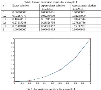
Example 1: Consider the following VIDE:
U′′ 𝑥 = 𝑒2𝑥− 𝑒𝑥 2(𝑥−𝑡)𝑈′ 𝑡 𝑑𝑡
0 Initial conditions 𝑈(0) = 0, 𝑈’(0) = 0.
The exact solution 𝑈 𝑥 = 𝑥𝑒𝑥− 𝑒𝑥+ 1. Table 1 shows the numerical results for this example with k=2, M=3 with error =10-3 and k=2, M=4, with error =10-4 are compared with exact solution graphically in fig.
Table 1:some numerical results for example 1 x Exact solution Approximat solution
k=2,M=3
Approximat solution k=2,M=4
0 0.00000000 0.00000001 0.00000001
0.2 0.02287779 0.02280000 0.02287000
0.4 0.10940518 0.10945544 0.10940544
0.6 0.27115248 0.25826756 0.27826756
0.8 0.55489181 0.54330957 0.55330957
1 1.00000000 0.99999995 0.99999998
Fig 1:Approximate solution for example 1
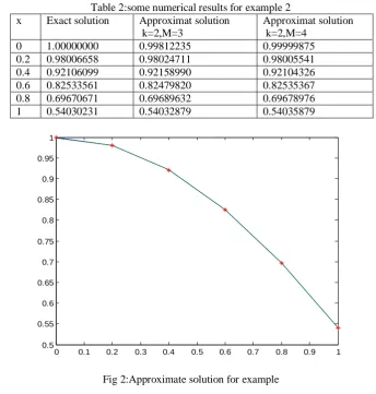
Example 2: Consider the following VIDE :
U(5) 𝑥 = −2 sin 𝑥 + 2 cos 𝑥 − 𝑥 + (𝑥 − 𝑡)𝑈𝑥 (3) 𝑡 𝑑𝑡
0 Initial conditions 𝑈(0) = 1, 𝑈’(0) = 0, 𝑈"(0) = −1, 𝑈3(0) = 0.
The exact solution 𝑈 𝑥 = cos 𝑥. Table 2 shows the numerical results for this example with k=2, M=3 with error=10-3 and k=2, M=4, with error =10-4 are compared with exact solution graphically in fig, 2.
0 0.1 0.2 0.3 0.4 0.5 0.6 0.7 0.8 0.9 1
Table 2:some numerical results for example 2 x Exact solution Approximat solution
k=2,M=3
Approximat solution k=2,M=4
0 1.00000000 0.99812235 0.99999875
0.2 0.98006658 0.98024711 0.98005541 0.4 0.92106099 0.92158990 0.92104326 0.6 0.82533561 0.82479820 0.82535367 0.8 0.69670671 0.69689632 0.69678976
1 0.54030231 0.54032879 0.54035879
Fig 2:Approximate solution for example
V. CONCLUSION
This work proposes a powerful technique for solving VIDE second kind using wavelet in collocation method comparison of the approximate solutions and the exact solutions shows that the proposed method is more faster algorithms than ordinary ones. The convergence and accuracy estimation of this method was examined for several numerical examples.
REFERENCES
[1] Asmaa A. A , 2014, Numerical, Solution of Optimal Control Problems Using New Third kind Chebyshev Wavelets Operational Matrix of Integration, Eng&Tech journal,Vol 32,part(B),1:145-156. [2] Tao. X. and Yuan. L. 2012. Numerical Solution of Fredholm Integral Equation of Second kind by
General Legendre Wavelets, Int. J. Inn. Comp and Cont. 8(1): 799-805.
[3] A.Barzkar, M.K.Oshagh, 2012, Numerical solution of the nonlinear Fredholm integro-differential equation of second kind using chebysheve wavelets, World Applied Scinces Journal (WASJ),Vol.18, N(12):1774-1782.
[4] E.Johansson, 2005, Wavelet Theory and some of its Applications.
[5] Jafari. H and Hosseinzadeh. H. 2010. Numerical Solution of System of Linear Integral Equations by using Legendre Wavelets, Int. J. Open Problems Compt. Math., 3(5): 1998-6262 .
[6] Shihab. S. N. and Mohammed. A. 2012. An Efficient Algorithm for nthOrder Integro- Differential Equations Using New Haar Wavelets Matrix Designation, International Journal of Emerging & Technologies in Computational and Applied Sciences (IJETCAS). 12(209): 32-35.
[7] M.Razzaghi & S.Yousefi. 2002. Sin-Cosine wavelets operational matrix of integration and it’s applications in the calculus of variations. Vol 33. No 10: 805-810.
[8] A.Arikoglu & I.Ozkol. 2008. Solution of integral integro-differential equation systems by using differential transform method. Vol 56,Issue 9.2411-2417.
[9] Arsalani. M. & Vali. M. A.,2011 Numerical Solution of Nonlinear Problems With Moving Boundary Conditions by Using Chebyshev Wavelets, Applied Mathematical Sciences,Vol.5(20): 947-964.
0 0.1 0.2 0.3 0.4 0.5 0.6 0.7 0.8 0.9 1