A space-probabilistic separation approach for Structure Static reliability analysis

ISSN (e): 2250-3021, ISSN (p): 2278-8719

Vol. 07, Issue 06 (June. 2017), ||V1|| PP 30-44

A space-probabilistic separation approach for Structure Static

reliability analysis

L. Ncib**, A. Manai*, H. Hassis*

Université de Tunis El Manar, École Nationale d’Ingénieurs de Tunis2_{, BP 37, Le Belvédère 1002, Tunis,} Tunisia

Abstract:- In mechanics, as in many scientific domains, information and data can be:deterministic (certainty known or with error - safety coefficient),probabilistic (random with known probability distribution),possibilistic (random known with an uncertainty factor on the reliability of the information. Parameters change in a known range, but the probability is unidentified).The probabilistic mechanical approaches aim to give an estimation of the solution when the information on the parameters of analyzed problem is uncertain.For some mechanical problems with probabilistic parameters, a constraint to be satisfied is added. In engineering design, the reliability analysis is an example of such constraint.In this paper, and for static probabilistic-reliability analysis, an approach reducing the size of numerical computing is proposed. It will be validated on static discrete and continuous systems having probabilistic parameters.

Keywords: probabilistic, reliability, model reduction.

I.

GENERAL INTRODUCTION: PROBABILISTIC ANALYSIS FOR THE

RELIABILITY

To improve the security level of mechanical components, a reliability analysis should be done from the first stage of the conception, mainly when the parameters are random or uncertain.In reliability analysis, choice or/and modification of parameters are made to satisfy some conditions. It leads to a large number of sensitive computations [1-7]. Remind that, the reliability analysis compares the security constraints (stress or displacement) with the resistance or displacement limits; needs versus resistance. As a global indicator, the probability of failure is calculated in which the need is greater than or equal to the resistance; [8-15].

A good approach should easily:

 takes into account the impact of uncertain or partially unknown parameters on the reliability constraints,  has the possibility to act (or to change) on theses parameters to satisfy theses constraints.

For a better risk management consideration, the analysis should be done at the beginning of the design phase. Moreover, the lack of information about these uncertainties can be a handicap for a good modeling of the studied systems.When the reliability constraints, with the probabilistic parameters, are considered in the mechanical problem formulation, a very large size problem or a large number of problems is obtained. In some cases or methods, it is recommended to reduce the number of parameters which can be obtained by coupling between the condensation methods and the reliability methods. First and second-order reliability methods (FORM and SORM, respectively) are famous approximation methods that estimate the probability of a failure event. These methods are useful in the uncertainty analysis of models with a single failure criterion. For a mechanical model with np basic random parameters, X=(x1, x2,….xnp), the objective of the reliability approach is

to estimate the probability of failure when the failure condition is not reached. Generally, it is defined by a function G(x1, x2,….xnp)<0. In the case of the limit state of displacement, as an example, the failure condition

can be defined as:

G(x1, x2,….xnp)=W(x1, x2,….xnp)-Wlim<0 (1)

where Wlim is an allowable displacement and W is the displacement at defined design location.

Then, in reliability analysis, the probability of failure is an important factor to be determined. It is defined by:

Pf = P(G(x1, x2,….xnp)<0)=P(W(x1, x2,….xnp)-Wlim<0) (2)

1_{Corresponding Author : [email protected]} 2

The probability of failure, even it can be written easily but it needs a big capacity of computer calculation. It can be estimated using some approximation methods, such FORM/SORM [3, 4]. By using a tangent (FORM), or by a parabolic (SORM) approximation of the function G at the failure point closest to the design point, the probability of failure can be determined as a simple function of failure point.

To obtain an approximation of the probability of failure, Bjerager [16] proposed the following step for FORM and SORM:

 The basic random variables x and the failure function, G, are mapped into a vector of standardized and uncorrelated normal variants u, as x(u) and g(u), respectively

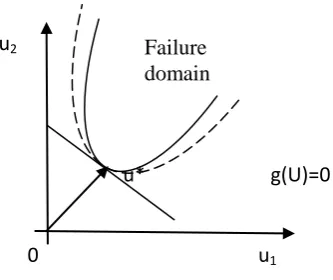
 The function g(u) is approximated by a tangent (FORM) or a parabolic (SORM) at the failure point u* closest to the origin; (see Figure 1)

 The probability of failure is then calculated as a simple function of u*

Compared to Monte Carlo methods, FORM and SORM can be computed easily, especially for scenarios corresponding to low probabilities of failure. By its higher-order approximation, SORM is more accurate than FORM but it needs more intensive computer operations.Even if FORM and SORM are based on a simple mapping of the failure function onto a standardized set, the minimization of the function G involves significant computational effort for nonlinear problems. Additional efforts are necessary when the problem contains a multiple failure criteria; the determination of the probability of failure needs a simultaneous evaluations. These methods also impose some conditions on the joint distributions of the random parameters, thus limiting their applicability.

Figure 1. Principle of the approximation methods FORM/SORM

The presented work is not a classical condensation method; the condensation is obtained by a projection on a set of representative functions. Finally, the paper deals with the following aspects:Developing a strategy for treatment of imprecision for assessing the probability of structures failure by coupling the probabilistic and mechanical methods;Analyzing the methods of coupling between condensation methods and reliability methods in order to reduce computational cost.

Failure domain

x

x

P*

1

0

G(X)=0

Failure

domain

u

u

u*

0

II.

GENERAL PRESENTATION OF THE SPACE-PROBABILISTIC SEPARATION

APPROACH

In reliability of mechanical system, the determination of the safe area (where a criterion is satisfied) leads to a large numerical problem(s). The first objective is to reduce the problem’s size; [18-23]. The optimum choice of new parameters optimizing the cost or the technical design and fabrication is a second objective. To reach the two objectives, accelerator methods should be used and this work is one of them. The present approach is based on a separation variables method and on a projection on a specific set of representative functions. The research of a solution by separating variables is not a new proposal; the space-time separated representation is a famous example. Here proposed a new application of the decomposition on a separated variable functions but at space-probabilistic domains.Even the approach is valid for any linear probabilistic application; mechanical applications are chosen to valid this approach. Consider that each probabilistic variable Vi follows its law (seen in appendix two examples of classical laws) defined by its density distribution and its

cumulative distribution function Pi(vi) which can be inversed to vi(Pi).

Consider that a static problem containing np probabilistic parameters, Vi, defined by a linear problem:

F X P P K F X P v K noted F X P v P v K p n i i p n p n    ). ...., ( )). ( ( ; )). ( ),...., ( ( 1 1 1 (3)

K is the stiffness matrix issued from the space discretization and contains np probabilistic parameters. Each

probabilistic parameter number i, vi, has its own probabilistic law. F is the force vector and also could depend of

probabilistic parameters.

Let  _j a known and chosen probabilistic representative functions (it is not established that it is a base); j varies from 1 to at last np. In section 3, 4 and 5 of this paper, it will be explained how to choose the functions for

each specified problem. In some cases,  _j can depend only of one parameter, and then the number of the used functions is np. For other cases,  j can depend of different parameters, and then the number of the used

function is less than np.;

'

p

n will denote the maximum number of functions.

By using the separation variables approach and by decomposition the unknown parameters X on the representative set of functions,  _j, the solution X is written as the following decomposition:



X (4)

Using the decomposition 4, equation 3 is written as:

F X P K p n j j j i             ' 1 ). ( (5)

Multiplying equation 5 by any function _k and integrates it in the probabilistic domain (from 0 to 1) leads to

equation 6.   ' 1 0 1 1 0 1 0 1 ' 1 1 0 1 ; .. . .. .. . ). ( .. _p p n k p n k p n j j j

i X dP dP F dP dP k to n

P

K    

            

_

_







For many cases, the integration defined by equation 6 is formal (expressions are analytical). Equation 6 leads to

'

p

n associated problems, as expressed by 7:

' ' 1 1 ; _p k p n j j

kjX F k to n

K  

 

(7)

                                                                                              ' ' 1 1 * * * * . . . . p n k p n j p kn kj k F F X X X K K K (8)

With:  _{ }









1 0 1 1 0 1 0 1 1 0 .. ) ( .. ; .. . ) ( .. p n k i k p n k j i

kj K P dP dP F F P dP dP

K (9)

The dimension of K_kj is the same of K. The Xj are solved and the probabilistic solution is obtained by the

recombination defined by:



X (10)

Remarks: compared to a direct approach, and suppose that the probabilistic domain of each parameter (between 0 and 1) is divided into only 10 intervals, the reduction of the size of calculation is:

• np=1 : reduction: 90% (from 10 problems with n*n dimensions to 1 problem with n*n)

• np=3: reduction: 97,3% (from 1000 problems with n*n to 1 problem with 3n*3n)

• np=4: reduction: 99,36 % (from 10000 problems with n*n to 1 problem with 4n*4n)

• np=k: reduction: .100 %

10 1 3          k k

(from 10 k problems with n*n to 1 problem with kn*kn)

The presented approach is first applied for discrete system (section 3) and for beam structure (section 4). Even the examples are academic, the accuracy of the method will be demonstrated.

III.

PROBABILISTIC DISCRETE SYSTEM APPLICATIONS

Notation: for all discrete examples, k is a stiffness, m is a mass, f is a force and x is a local displacement. The probabilistic parameters are defined by their mean or expectation of the distribution and their standard deviation. Their probability (cumulative distribution function) P(k) is then estimated and its inverse function k(P) is calculated. For discrete systems, solutions are computed using the maple tools.

3.1. A Two-DOF discrete system with two probabilistic parameters

Consider two degrees of freedom spring-masse system, shown in figure 2. The mean or expectation of the distribution and the standard deviation of k1 and k2 are respectively: μk1= 2E10 N/m, σk1 = 4E9 N/m, μk2= 1E10

N/m, σk2 = 3E9 N/m. The forces are f1=3.5E7 N and f2=3.5E7 N.

Figure 2. A two degrees of freedom (DOF) system with 2 probabilistic parameters

The static equilibrium equations are written as follows:

                      2 1 2 1 2 2 2 2 1 . f f x x k k k k k

or K.X  F (11)

Two functions are used here and defined by:

f1

f2

m1

m2

k1

k2

) ( ) ( ; ) ( ) (

2 2

2 2

2 1 1

1 1

1

P k P P

k

P k k

 

 



 (12)

The analytical displacements x1 and x2 are superposed to those obtained by the RPR model in figure 3 and 4.

Figure 3. Displacement x1 Figure 4. Displacement x2

as a function of the cumulative distribution function P1(k1) and P2(k2)

The Relative error (%) for the displacements x1 and x2 as a function of the cumulative distribution function

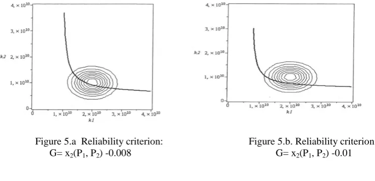
P1(k1) and P2(k2) are less than 10-6 %. As example of reliability criterion, the displacements (x1 and x2) should be

less than 0.008 m and 0.01 m, respectively. The displacement x1 is always less than the limit; the limitation for

the displacement x2 is respectively represented by figures 5.a and 5.b.

Figure 5.a Reliability criterion: Figure 5.b. Reliability criterion:

G= x2(P1, P2) -0.008 G= x2(P1, P2) -0.01

3.2. Two-DOF lumped parameter system with two different probabilistic laws

Consider the same example described in the section 3.1 but let k1 be a uniform distribution law defined by:

ak1=8E9 N/m and bk1=3.2E10 N/m, and let k2 be a Gaussian probabilistic law defined by μk2= 1E10 N/m, σk2.=

3E9 N/m. The forces are f1= f2= 3.5E7 N.

The relative error between the analytical solution and RPR solution is around 1E-6.

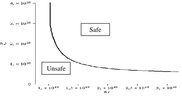
Figure 6.a. safe and unsafe area are represented as a function of the probabilities

Figure 6.b safe and unsafe area are represented as a function of the of stiffness

3.3. A curious example: Two-DOF lumped parameter system with one probabilistic and one deterministic parameters

Consider the same example described in the section 3.1 but let k1 be a determinist parameter, k1=2E10 N/m, and

let k2 be a probabilistic one defined by μk2= 1E10 N/m, σk2.= 3E9 N/m. The forces are f1= f2= 3.5E7 N.

Figure 7. Two degrees of freedom (DOF) system

First, only one probabilistic function is used. The displacements x1 and x2 (exact and done by this approach) are

superposed in figures 8 and 9. The relative error is important.

Then, using a special function associated to a deterministic parameter, the solution is close to the exact one;

f1

f2

m1

m2

k1

k

x1

x2

Deterministic parameter

Probabilistic parameter

Safe

Unsafe

Unsafe

Figure 8. Superposition of x1 (in %) Figure 9. Superposition of and x2 (in %)

exact and done by one function

Figure 10. Superposition of x1 Figure 11. Superposition of x2

*** exact and ____ done by two functions

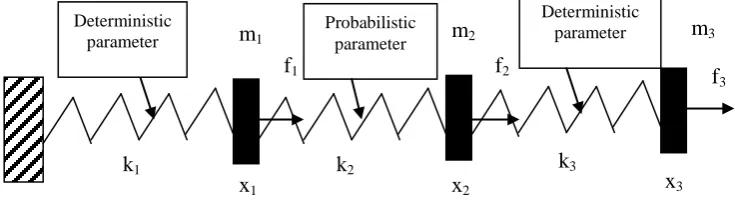
3.4. A confirmation of the necessity of one function associated to all deterministic parameters: three-DOF discrete system with only one probabilistic parameter

Consider a three degrees of freedom spring-masse system, as shown in figure 12. The forces are f1= f2=

f3=3.5E7 N.

k1 and k3 are deterministic parameters with k1=2E10 N/m and k3=3E10 N/m; k2 is a probabilistic one defined by

μk2= 1E10 N/m, σk2.= 3E9 N/m.

Figure 12. A three degrees of freedom (DOF) system

Here, two probabilistic base functions are used: the first one corresponds to all constant parameters and the second one corresponds to the probabilistic parameter.

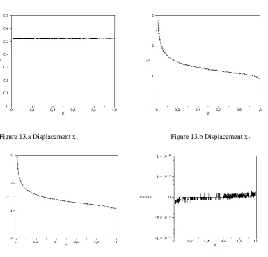
The superposition of the displacements x1, x2 and x3 and an example of the relative error of x2 are represented

respectively in figure 13.a to 13.d.

x1

x2

x3

Deterministic parameter

Probabilistic parameter

f1

f2

m1

m2

k1

k2

f3

parameter

m3

Figure 13.a Displacement x1 Figure 13.b Displacement x2

Figure 13.c Displacement x3 Figure 13.d Relative error of x2, as example

IV.

FRAME SYSTEM APPLICATIONS

a.

The implementation of the approach was performed on the Matlab numerical code, especially for a 2D beam finite element defined by its probabilistic parameters: the Young modulus, E, and the two section parameters a and b; figure 14.

Figure 14. Beam with rectangular section

The results obtained by this approach are compared with those obtained by Monte Carlo (MC) simulations. Monte Carlo methods (or Monte Carlo experiments) are a broad class of computational algorithms that rely on repeated random sampling to obtain numerical results. The Monte Carlo (MC) method calculates functions of the form E (X) = μ, where X is a real and vector random variable. It is based on the generation of numerous pulling of independent copies of X and the strong law of large numbers:

𝜇 = lim𝑛→+∞

1

𝑛( 𝑋1+ … + 𝑋𝑛 ≔ lim𝑛→+∞𝜇 𝑛 (13)

The precision of the result is measured by the probability of being wrong. Called "α% Confidence Interval, C-I". It is of the form 𝜇 𝑛− 𝜀, 𝜇 𝑛+ 𝜀 , in which it is safe to α%. It is guaranteed by:

𝑃 𝜇 − 𝜇 𝑛 > 𝜀 < 1 − 𝛼 (14)

a

b

The central limit theorem indicates that 𝑛

𝜎 𝜇 𝑛− 𝜇 converges to a centered and reduced Gaussian distribution, with 𝜎2_{= 𝑉(𝑋). We deduce that:}

𝑃 𝜇 − 𝜇 𝑛 > 𝜀 ~ 1 2𝜋 𝑒 −𝑥 2 2 +∞ 𝜀 𝑛 𝜎

𝑑𝑥 (15)

When it was considered that 1

2𝜋 𝑒

−𝑥 2 2

+∞

𝑎 𝑑𝑥 = 1 − 𝛼, then the α% confidence interval is given by:

𝜇 𝑛− 𝑎 𝜎

𝑛 , 𝜇 𝑛 𝑛+ 𝑎 𝜎

𝑛 (16)

When σ is unknown, it is replaced by the sample variance of the observations noted 𝜎𝑛 and given by: 𝜎𝑛2=

1

𝑛−1 𝑋𝑖− 𝜇 𝑛 2 𝑛

𝑖=1 (17)

4.1. First analyzed structure

Let a frame structure constrained at A and loaded at B by a force equal to F=5E5 N, as indicated in figure 15.

Figure 15. The analyzed structure

Three cases are analyzed, as defined by Table1:

Case 1 Case 2 Case 3

(E,a) probabilistic (E,b) probabilistic (E,a,b) probabilistic

(E)= 2E11 N/m2

(E)= 2E10 N/m2

(a)= 0.035 m (a)= 0.0035 m; b=0.35

(E)= 2E11 N/m2

(E)= 2E10 N/m2

(b)= 0.35 m; (b)= 0.035 m a=0.035

(E)= 2E11 N/m2

(E)= 2E10 N/m2

(a)= 0.035 m; (a)= 0.0035 m (b)= 0.35 m; (b)= 0.035 m Representative set functions

) ( ) ( ) , ( 1 a E a E a E P a P E P

P   

 ) ( ) ( ) , ( 1 b E b E b E P b P E P

P   

   ) ( ) ( ) , ( 3 3 2 b E b E b E P b P E P

P   

 ) ( ) ( ) ( ) , , ( 1 b a E b a E b a E P b P a P E P P

P    

   ) ( ) ( ) ( ) , , ( 3 3 2 b a E b a E b a E P b P a P E P P

P    



Table1. Definition of different analyzed cases

It is assumed that the reliability is defined by a criterion on the deflection W, at the node B, which should be smaller than a limited displacement wmax = -0.3m. The objective function can be defined as follows:

G = W − wmax (18)

The objective is to calculate the probability of default, Pf, defined by:

Pf(G = W − wmax < 0) (19)

Figure 16 (respectively 18) shows the evolution of the deflection at node B as a function of cumulative

distribution functions of the probabilistic parameters of case 1 (respectively of the case 2).

Figure 16. Case 1: Evolution of the displacement at B as a function of cumulative distribution functions of P(E) and P(a)

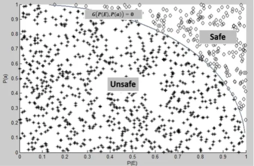
Figure 17. Case 1: Safe and unsafe areas

Figure 19. Case 2: Safe and unsafe areas

Figure 20.Case 3: Safe and unsafe areas

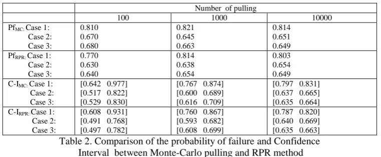
The failure probability, Pf, was calculated by the RPR model (PfRPR), the validation of this probability

is made by a comparison with results obtained by the Monte Carlo method (PfMC).Table 2 compares the

probability of failure and the Confidence Interval (C-I) between Monte-Carlo pulling and RPR method. Table 2 is done with =0.95: we are sure, with 95% of confidence, that the Pf will be in the C-I.

Number of pulling

100 1000 10000

PfMC: Case 1:

Case 2: Case 3:

0.810 0.670 0.680

0.821 0.645 0.663

0.814 0.651 0.649 PfRPR: Case 1:

Case 2: Case 3:

0.770 0.630 0.640

0.814 0.638 0.654

0.803 0.654 0.649 C-IMC: Case 1:

Case 2: Case 3:

[0.642 0.977] [0.517 0.822] [0.529 0.830]

[0.767 0.874] [0.600 0.689] [0.616 0.709]

[0.797 0.831] [0.637 0.665] [0.635 0.664] C-IRPR: Case 1:

Case 2: Case 3:

[0.608 0.931] [0.491 0.768] [0.497 0.782]

[0.760 0.867] [0.593 0.682] [0.608 0.699]

[0.787 0.820] [0.640 0.669] [0.635 0.663]

Table 2. Comparison of the probability of failure and Confidence Interval between Monte-Carlo pulling and RPR method

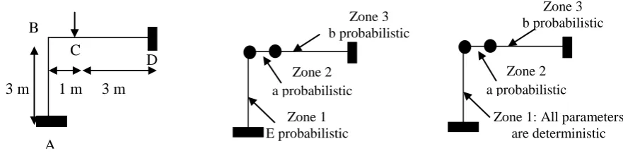
Figure 21. Analyzed structure and the two studied cases

AB: zone 1 BC: zone 2 CD: zone 3

Case 1 E1=Probabilistic

a1=0.035

b1=0.35

E2=2E11

a2= Probabilistic

b2=0.35

E3=2E11

a3=0.035

b3= Probabilistic

Case 2 E1=2E11

a1=0.035

b1=0.35

E2=2E11

a2= Probabilistic

b2=0.35

E3=2E11

a3=0.035

b3= Probabilistic

Tables 4. Different analyzed cases

The case 1 is analyzed for its probabilistic parameters at different zones of the structure. The case 2 is analyzed for its deterministic zone and the necessity or not of the use of a special function as the examples of the sections 5.2 and 5.3. For the case 1, the classical representative functions are used and a good result is obtained showing the possibility of the use of the present method for non global probabilistic parameters and a different local probabilistic parameters; see figure 22.

Figure 22. Case 1. Safe and non safe area for a limit displacement 0.6 m at point C

For the case 2, first only probabilistic classical representative functions are used and then a special function associated to all deterministic parameters is used. Figures 23.a and 23.b show that the use of the special function gives very good results.

B

A

C

!

%

%

%

%

%

%

%

%

%

%

%

%

%

%

%

%

%

%

%

%

%

%

%

%

%

%

%

%

%

%

%

%

%

ù

ù

m

3 m

D

1 m

3 m

Zone 3 b probabilistic

Zone 1 E probabilistic

Zone 2 a probabilistic

Zone 1: All parameters are deterministic

Zone 3 b probabilistic

Figure 23.a. Without using a special function f igure 23.b. With using a special function

V.

EMPIRICAL METHOD OF CHOOSE OF REPRESENTATIVE FUNCTIONS

From examples, and it is not demonstrated, the best set representative functions are obtained by the independent function obtained from the inverse of the elementary matrix. As follows, the set functions associated to classical examples are given.

5.1. Example 1: Discrete system

The discrete system of the section 5.1 is defined by its stiffness matrix and its inverse:

                         2 1 1 1 1 1 2 2 2 2 1 1 1 1 1 1 ; k k k k k K k k k k k K (20)

The independent functions (

1 1 k , 2 1 k

) represent the representative set of functions.

The discrete system of the section 5.3 is defined by its stiffness matrix and its inverse:

                                          3 1 1 1 1 1 1 1 1 1 1 1 1 1 1 ; 0 0 2 1 2 1 1 2 1 2 1 1 1 1 1 1 3 3 3 3 2 2 2 2 1 k k k k k k k k k k k k k k K k k k k k k k k k K (21)

The independent functions (

1 1 k , 2 1 k , 3 1 k

) represent the representative set of functions.

5.2. Example 2: 2D in plane stress

Let a system with three unknown parameters (11, 22,12) with two probabilistic parameters E and and

related by the following linear system (2D in plane stress). The inverse matrix gives an idea about the set of representative functions.                                               12 22 11 2 2 2 2 12 22 11 . 1 2 0 0 0 1 1 0 1 1              E E E E E                                          12 22 11 12 22 11 . 1 2 0 0 0 1 0 1          E E E E E (22)

It is clear that the two functions

E 1

and

E



are independent and can be a representative set of functions. It is

confirmed that any independent combination can be a set representative functions, as:

E   1 and E   1 .

Safe

Safe

Unsafe

5.3. Example 3: 2D beam element

For a 2D beam, the elementary matrix and its inverse are:

𝐸𝑎𝑏

𝑙 0 0

0 𝐸𝑎 𝑏3

𝑙3 −

𝐸𝑎 𝑏3 2𝑙2

0 −𝐸𝑎 𝑏3 2𝑙2

𝐸𝑎 𝑏3

3𝑙

𝑙

𝐸𝑎𝑏 0 0

0 4𝑙3 𝐸𝑎 𝑏3

6𝑙2 𝐸𝑎 𝑏3

0 6𝑙2 𝐸𝑎 𝑏3

12𝑙

𝐸𝑎 𝑏3

(23)

The two representative functions are:

) ( ) ( ) ( ) , , ( 1

b a E

b a E b

a E

P b P a P E P P

P    

 ;  

) ( ) ( ) ( ) , , (

3 3

2

b a E

b a E b

a E

P b P a P E P P

P    

 (24)

Remark: for any other finite element, it is suggested to inverse the elementary finite element matrix (the inversed part) and the independent functions will be the representative set functions.

VI.

CONCLUSIONS AND PERSPECTIVES

For a reliability analysis with probabilistic parameters, classical approaches lead to a problem with a large size. Reducing its size without any alteration of the solution is recommended for a good design.Here presented a general theory for static approach for reliability probabilistic analysis. For static problem, the solution is projected on well-chosen representative set of functions and an approximated solution is obtained. The equivalent problem reduces the size problem.The Reduction Probabilistic Reliability (RPR) approach, here described, is applied for static probabilistic discrete and frame examples. Discrete and frame static systems are analyzed and compared with exact solutions or issued from Monte-Carlo pulling analysis.As perspectives, these approach can be extended to possibilistic evolution parameters and to dynamic analysis in frequencies domain.

VII.

ACKNOWLEDGEMENTS:

This work is supported by:The European MOBIDOC/PASRI program, ESI Tunisia, ESI France, Astrium.

REFERENCES

[1] D. Dubois, H. Prade, P. Smets, New semantics for quantitative possibility theory. In 2nd International Symposium on Imprecise and their Applications Ithaca, New York, 2001

[2] O. Dessombz, F. Thouverez, J.-P. La n , L. J z quel, Analysis of mechanical systems using interval computations applied to finite element methods, Journal of Sound and Vibration 239(5) 949-968, 2001.

[3] O. Dessombz. Analyse dynamique de structures comportant des paramètres incertains. Thèse de doctorat, Ecole centrale de Lyon 2000

[4] R. M. Moore. Interval Analysis. Prentice-Hall, 1966.

[5] R. M. Moore. Method and applications of Interval Analysis. Studies in Applied Mathematics (SIAM), 1979.

[6] J. Rohn. On overestimations produced by the interval gaussian algorithm. Technical Report 690, Institute of Computer Science, Academy of Sciences of the Czech Republic, oct 1996.

[7] A. D. Dimarogonas. Interval analysis of vibrating systems. Journal of Sound and Vibration, 183(4):739-749, 1995.

[8] D.M. Frangopol, Structural Optimization Using Reliability Concept. Journal of Engineering Structures, ASCE, v. 111, p. 2288-2301, 1985.

[9] M. Lemaire. Reliability and mechanical design. Reliability Engineering and System Safety, 55 :163-170, 1997.

[10] R. Nakib. Deterministic and reliability based-optimization of truss bridge. Computers and Structures, 65(5) :767-775, 1997. [11] Breitung K, Casciati F, Faravelli L. Reliability based stability analysis for actively controlled structures. Engineering Structure,

20(3): 211-215, 1998.

[12] R. E. Melchers. Structural Reliability Analysis and Prediction. Wiley, second edition, 1999.

[13] O. Ditlevsen. Generalized second moment reliability index. Journal of Structural Mechanics, pages 453 472, 1979.

[14] C.G. Bucher and U. Bourgund. A fast and efficient response surface approach for structural reliability problems. Structural Safety, 7:57 66, 1990.

[15] P.H. Waartsa, A.C.W.M. Vrouwenveldera, Stochastic finite element analysis of steel structures. Journal of Constructional Steel Research, 52 :21-32, 1999.

[16] P. Bjerager, and S. Krenk, (1989). ”Parametric Sensitivity in First Order Reliability Theory.” J. Eng. Mech., 115(7), 1577–1582 [17] C. Cremona, Y. Gao, The possibilistic reliability theory: theoretical aspects and applications, Structural Safety, 19(2) 173-201,

1997.

[18] J.P. Lombard, Contribution la réduction des modèles éléments finis par synthèse modale, Thèse de doctorat en sciences pour l'ingénieur, Université de Franche-Comté, 1999.

[19] MASSON G., Synthèse modale robuste adaptée à l’optimisation de modèles de grande taille, Thèse de doctorat en sciences pour l'ingénieur, Université de Franche-Comt , 2003.

[20] BALM S E., Parametric families of reduced finite element models. Theory and applications, Mechanical Systems and Signal Processing, vol. 10(4), p.381-394, 1996.

[22] N. Rabhi, M. Guedri, H Hassis and N. Bouhaddi. Structure dynamic reliability: A hybrid approach and robust meta-models, Mechanical Systems and Signal Processing, Volume 25, Issue 7, October 2011, Pages 2313-2323

[23] U. Kirsch, S. Liu, Exact structural reanalysis by a first order reduced basis approach, Structural optimisation 10, 153-158, Springer-Verlag, 1995.

[24] [24] I. Tani, Fiabilité et robustesse en dynamique des bâtiments, 2005.

Appendix: Basic examples of probabilistic laws

Here is characterized, through some examples, the probabilistic parameters and theirs relative laws. As examples, two practical used probabilistic law parameters are presented and characterized.

Gaussian Law distribution

Consider that variable vi follows the Gauss normal law which is defined by:

2 2 2 ) ( 2 1 ) ( i i i v i i

i v e

f        (1)

The parameter μi is the mean or expectation of the distribution (and also its median and mode). The

parameter σi is its standard deviation; its variance is therefore σi2.

For a generic normal distribution fi with mean μi and deviation σi, the cumulative distribution function is:

        _   ) 2 ) ( ( 1 2 1 ) ( i i i i i v erf v P   (2)

erf(x) is the related error function defined by: erf x e dt

x x t



It gives the probability that the value of a standard normal random variable Vi will not exceed vi. The inverse

expression v_i(P_i) of P_i(v_i) will be used to write the problem as a function of the cumulative distribution functions of variables. It can be obtained for all probabilistic laws.

Uniform Law distribution

The uniform law distribution is based on the continuous uniform distribution or rectangular distribution. It is a family of symmetric probability distributions such that for each member of the family, all intervals of the same length on the distribution's support are equally probable. The support is defined by its

minimum and maximum values: v_imin and v_imax .

The probability density function of the continuous uniform distribution is:

               max min max min min max 0 1 ) ( i i i i i i i i i i v v or v v for v v v for v v v

f (3)

The cumulative distribution function is:

                  max max min min max min min 1 0 ) ( i i i i i i i i i i i i i v v for v v v for v v v v v v for v