C a u s ali ty-b a s e d c o s t-e ff e c tiv e
a c ti o n m i ni n g
S h a m si n ej a d b a b ki, P, S a r a e e , M H a n d Blo c k e e l, H
h t t p :// dx. d oi.o r g / 1 0 . 3 2 3 3 /IDA-1 3 0 6 2 1
T i t l e
C a u s ali ty-b a s e d c o s t-e ff e c tiv e a c tio n m i ni n g
A u t h o r s
S h a m s i n ej a d b a b ki, P, S a r a e e , M H a n d Blo c k e el, H
Typ e
Ar ticl e
U RL
T hi s v e r si o n is a v ail a bl e a t :
h t t p :// u sir. s alfo r d . a c . u k /i d/ e p ri n t/ 4 8 1 8 5 /
P u b l i s h e d D a t e
2 0 1 3
U S IR is a d i gi t al c oll e c ti o n of t h e r e s e a r c h o u t p u t of t h e U n iv e r si ty of S alfo r d .
W h e r e c o p y ri g h t p e r m i t s , f ull t e x t m a t e r i al h el d i n t h e r e p o si t o r y is m a d e
f r e ely a v ail a bl e o nli n e a n d c a n b e r e a d , d o w nl o a d e d a n d c o pi e d fo r n o
n-c o m m e r n-ci al p r iv a t e s t u d y o r r e s e a r n-c h p u r p o s e s . Pl e a s e n-c h e n-c k t h e m a n u s n-c ri p t
fo r a n y f u r t h e r c o p y ri g h t r e s t r i c ti o n s .
Causality-based Cost-effective Action Mining
Pirooz Shamsinejadbabaki
1, Mohamad Saraee
2, and Hendrik
Blockeel
31
Electrical and Computer Engineering Department, Isfahan
University of Technology,Isfahan,Iran
2
School of Computing, Science and Engineering, University of
Salford-Manchester, Manchester, UK
3
Department of Computer Science, KU Leuven, Leuven, Belgium
January 19, 2013
Abstract
In many business contexts, the ultimate goal of knowledge discovery is not the knowledge itself, but putting it to use. Models or patterns found by data mining methods often require further post-processing to bring this about. For instance, in churn prediction, data mining may give a model that predicts which customers are likely to end their contract, but companies are not just interested in knowing who is likely to do so, they want to know what they can do to avoid this. The models or patterns have to be transformed into actionable knowledge. Action mining explicitly addresses this.
Currently, many action mining methods rely on a predictive model, obtained through data mining, to estimate the effect of certain actions and finally suggest actions with desirable effects. A major problem with this approach is that predictive models do not necessarily reflect a causal relationship between their inputs and outputs. This makes the existing action mining methods less reliable. In this paper, we introduce ICE-CREAM, a novel approach to action mining that explicitly relies on an automatically obtained best estimate of the causal relationships in the data. Experiments confirm that ICE-CREAM performs much better than the current state of the art in action mining.
1
Introduction
a considerable amount of extra work by domain experts. The more we can nar-row the gap between the patterns mined and the knowledge required to make decisions, the more effectively data mining can be used in real-life problems. Action rule mining is motivated by this observation.
Action Rules are a type of knowledge that explicitly describes how changes in variables that can be influenced affect some target attribute that cannot be influenced directly [1].
They are much easier to apply than, for instance, association rules, because they specify exactly what should be done. For example [2], consider an intelli-gent loaning system for a bank that contains customers data. A traditional DM pattern in this system can be a classification rule like: if sex = ’M’ and service = ’L’, then payback = ’False’. However, an action rule can be like: if sex = ’M’ and service changes from ’L’ to ’H’, then payback will go from ’False’ to ’True’. In many business contexts, the second rule expresses more directly use-ful knowledge. Take, for instance, churn prediction: the company is not merely interested in predicting which customers it is going to lose, it wants to know what can be done to avoid this.
Action Mining (AM) is the process of learning action rules from data. Not much work has been done in this area up till now. Existing work includes Yang et al.’s method for learning actions from decision trees [3, 2], and several ver-sions of Ras et al.’s DEAR system for discovering action rules [4, 5, 6]. In all of these methods, input data is in the form of a set of attribute-value pairs for each object. Furthermore, a certain profit is associated with specific values of one particular attribute, called the target attribute. These methods then try to uncover existing associations between the target attribute and other attributes, and use these associations for finding the most beneficial actions. The main difference between these methods is in the technique by which they find asso-ciations. For example, Yang’s method uses decision trees, while DEAR 2 uses classification rules.
Despite all innovations presented in existing AM methods, they suffer from an important drawback: they implicitly rely on the assumption that the avail-able models (decision trees, association rules) are causal. It is well-known from statistics that association or correlation does not imply causation. Even though the learned models do not merely express the existence of a correlation, but its nature (in the form of a predictive function), they suffer from the same problem. If a function f :X →Y learned from a data set is found to be accurate, this means that, when weobserveX =xin a new object, we can accurately predict that Y = f(x); but if we manually change the object’s X value to X = x′,
there is no guarantee thatY changes intof(x′); in fact,Y may not be affected
at all. Basically, the joint distribution over(X, Y) of objects with a manually changedX differs from that of the observed objects in the training set, therefore the training set is not representative for these and there is no guarantee that models learned from it will be accurate in this new distribution.
long as its input consists of a C value observed under normal conditions, but if C is artificially increased by a promotional campaign, the model will tend to overestimateT. In cases like this, if a high temperature is desired, existing action rule mining algorithms would suggest to increase ice cream consumption, which obviously will have no effect.
The main contribution of this paper is a method that proposes actions based on causal relationships between attributes. The method relies on causal net-works (CNs), which are a powerful tool for representing causal relationships and performing inference on them. In particular, they correctly infer the effects of interventions (externally induced changes of values), which is exactly what we need here.
One might argue that such causal networks are rarely available in practice, when mining a database. However, one can try to construct them automatically from the data. There has been a lot of work on learning causal networks from data, starting with the foundational work of Pearl et. al. [7] and Spirtes et. al. [8]. They have shown that causal relationships can be inferred correctly under specific (but not under all) circumstances. This raises the following questions. Given a database, can we learn a causal network that is sufficiently accurate to be useful for action mining? And exactly how can such a causal network be used in this context? These are the questions we try to answer in this paper. They have not been studied before in action rule mining, and they pose a number of specific challenges that have not been addressed in the literature on causal networks, as will become clear later on.
In this text, we consider two scenarios. In the first scenario, which is mostly hypothetical but useful as a reference point, we assume that a correct causal net-work is available for the data. We present a method called Causal Relationship-based Economical Action Mining (CREAM) that, given an object and the causal network, predicts optimal (i.e., maximally cost-effective) actions. In the second, more realistic, scenario, we assume the causal network is not known. In that case, we can try to learn it from the data. This is a difficult task, and it is known that the correct network cannot be learned under most circumstances, but algorithms exist that return a partial network as a best possible estimate. A well known example is IC (Inductive Causation) [9]. ICE-CREAM (IC-enabled CREAM) refers to the complete approach of first running an inductive causa-tion algorithm (IC or one of its variants), then CREAM. This approach requires extending CREAM so that it can handle partial, rather than complete, causal networks.
The novel approach is computationally more intensive than some existing approaches, so the question is how much can be gained by using it. We ex-perimentally evaluate this on a number of datasets, comparing ICE-CREAM to the state of the art (which uses models that are not necessarily causal). The comparison shows that taking induced causality into account results in much better action recommendations.
in Section 4. We describe the core of our approach, the CREAM method, in Section 5, and the full method, ICE-CREAM, in Section 6. In Section 7, we experimentally compare our methods with Yang et al.’s method, testing them on different data sets. Finally, in Section 8 we conclude and discuss perspectives of causality-based action mining.
2
Related Work
Action mining is part of a subdomain of data mining called Actionable Knowl-edge Discovery (AKD), which is concerned with finding patterns that are not only interesting but also actionable, preferably with minimal further effort re-quired of domain experts. Piatetsky-Shapiro and Matheus[10] define a pattern as actionable if the user can act upon it to gain some advantage in the appli-cation domain. Although actionability could be considered a standard require-ment in data mining (it is roughly the same as “usefulness”, and no one wants to find useless patterns), most traditional systems do not explicitly maximize some well-defined actionability criterion, and the patterns they return do not explicitly express desirable actions: further inference is needed to identify those. We can categorize the existing work in AKD in different ways. A first di-chotomy relates to whether a standard or novel type of patterns is returned. Some methods (e.g. [11]) define a measure of interest called actionability, and filter patterns resulting from traditional methods based on this measure. Other methods try to learn a new type of knowledge, often calledaction rulesor simply
actions, from data. We here focus on the second type.
Assume objects are described by a set of attributes. An action is an exter-nally induced change of value of one attribute. Such an action can be taken with the goal of changing the state of the object into a desirable state. An action rule is an if-then rule that predicts the effect of applying certain actions under particular conditions. We define action mining as the process of finding desirable actions (for a given object), or finding rules that can predict desirable actions, by analyzing data. Following terminology from predictive modeling, we call methods that predict desirable actions for a given object transductive, and methods that learn action rules (which can afterwards be used to predict actions),inductive.
One of the first efforts towards action mining is the work by Ras et al.[1]. Their goal was to know “what actions should be taken to improve the prof-itability of customers”. They define the concept of action rules, distinguishing between flexible attributes, of which the value can be changed directly, and stable attributes, which cannot be changed directly. Valid actions consist of changing the value of a flexible attribute. This work led to the definition of a system called DEAR, which in successive work [4, 5, 6, 12] was developed into a full-fledged system that includes handling of missing values, outlier detection, and more.
the flexible attributes.
Tzacheva et al.[14] also use the influence matrix for finding action paths which are a sequence of actions. Characteristic for these approaches is that they require background knowledge (the influence matrix) that is not learned from the data, but assumed to be known. This reduces their applicability. We call these methods informed, as opposed to uninformed methods such as the DEAR series.
He et al.[15] present an Apriori-like method for learning action rules that takes into account the cost of action rules in addition to their support and confidence. Yang et al. [3, 2] present a method that first learns a decision tree from previous data and then uses the tree for finding the most profitable action for upcoming cases. Characteristic for these approaches is that a cost is associated with each action, which will be subtracted from the eventual profit obtained. The goal is then to find the set of actions that maximizes the net profit. One could call this “economical action mining”. Obviously, the setting with costs generalizes over that without costs (one could simply set all action costs to zero).
The method we propose in this paper is transductive (it predicts actions but does not yield generally applicable action rules), uninformed, and uses costs. From this point of view, the most closely related work is that of Yang et al. We therefore discuss it in more detail.
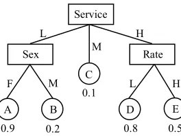
Yang et al.’s method first learns a decision tree, then analyzes the tree to find the optimal actions for each object. As the first step is pretty standard, we here focus on the second step. We illustrate it on the example decision tree in Fig. 1 [2], which represents a simplified decision tree built from customer profiles in a bank. The number below each leaf node is the probability that a random object in that node is in some desired state. This probability is estimated from past data. In Yang’s method, an action on an object is defined as a set of attribute value changes that moves an object from one leaf node to another one in the decision tree. For example, consider an instance(Service= L, Sex =
M, Rate = L). It is in leaf node B, but if Service were H instead of L, it would be in node D, in which the probability of being in the desired state is higher. It is therefore assumed that the action(service, L →H) will increase the probability that the customer is in the desired state.
Yang et al. associate a fixed profit p with the desired state, define the expected profit in a leaf as the proportion of cases in that leaf in the desired state, multiplied byp, and define the net profit of an action as the difference in expected profit between the from-leaf and the to-leaf, minus the cost of the action. A leaf-node search algorithm then selects for each object the action with maximum net profit.
as-Figure 1: A sample decision tree of customer profiles
sociation rules are not action rules by themselves, but could be post-processed using methods such as DEAR. To our knowledge, such an approach has never been tried in the field of action mining. The approach we propose here is an alternative to it that relies on more recent results in mining causal relationships. In the causal network literature, the focus has largely been on the challenging task of learning causal networks from data. Pearl’s seminal work [7] has given rise to a large number of algorithms that try to learn such networks. It is well-known how probabilistic inference in such networks can be done. In the context of action rule mining, however, new types of problems arise, which are of a more practical nature and which have not been considered in the causal networks literature:
1. Given a desirable state for one variable, and costs associated to actions that change the value of a variable, what is the most economical way of causing the target variable to take that value? This corresponds to optimizing the expected value of a function of some variables in the causal network.
2. The causal network derived form the data is often only partial; not all causal directions can typically be determined. The answer to question 1 can therefore only be computed by making additional assumptions or approximations. How well can the question be answered, when this is taken into account?
3. How can action rules be derived from the given data? An action rule is a generally applicable rule that states under what circumstances which vari-ables should be changed. These action rules can in principle be obtained by computing the answer to question 1 under many different circumstances, then learning rules from all these answers.
[image:7.612.239.371.74.173.2]3
The learning setting
As terminology and definitions in the literature vary somewhat, we here formally define concepts as they are used in this paper.
The input data for action learning is observational and in tabular form. Each column represents an attribute and each row an object. We assume there aren objects andm attributes. We write an object’s state as(A1 =a1, A2 =
a2,· · ·, Am =am), with each Ai an attribute and ai a value from its domain
Dom(Ai). Given an objecto, its value for attributeA is written asA(o). We assume there are no missing values.
We assume that all attributes are discrete; this is not a strong limitation, as real-valued attributes can always be discretized before applying the method. A denotes the set of all attributes in the system. One particular binary attribute is called the target attribute, and denoted byT. One ofT’s values is called the goal, denoted bytg; with this goal a profitpg>0is associated. With the other
value ofT a profit of 0 is associated.
An action is a structure of the form (A, a→ a′), with A a non-target
at-tribute anda, a′ ∈Dom(A). It corresponds to changing the value of attribute
A from a to a′ by means of an external intervention. With each action α a
costC(α) is associated. An action(A, a→a′) iscompatible with an object if the object’s value for A equals a. When an action α is applied to an object
o, we write the resulting state as oα. Note that, while an action(A, a →a′)
directly changes only A, this change may in turn cause changes to other at-tributes besidesA, according to the causal relationships that exist in the data. So, given an objectoand an actionα= (Ai, a→a′), there is no guarantee that
Aj(oα) =Aj(o)for eachj 6=i. Note that no additional cost is associated with
these indirect changes, only the action itself has a cost.
An action set Γ is a set of actions in which each attribute occurs at most once. An action set is compatible with an object if all its actions are compatible with it. Given an objecto and a compatible action setΓ = {α1, α2, . . . , αk},
we defineoΓ =oα1α2· · ·αk. It denotes the state of objecto after applying all
actions too. We define the cost of an action set asC(Γ) =Pα∈ΓC(α).
The net profitnp of an action set and an objecto is defined as np(Γ, o) =
pg−C(Γ)ifT(o)6=tg andT(oΓ) =tg, andnp(Γ, o) =−C(Γ)otherwise.
We define the task ofeconomical action miningas follows: Given an object space O = Dom(A1)× · · · ×Dom(Am), a data set D ⊆ O, a set of possible
actions and their associated costs, a target attributeT with associated goaltg
and profitpg, and a set of objectsO (which may or may not overlap with D),
find for eacho∈O an action setΓo such thatPo∈Onp(Γo, o)is maximal. It is useful to look back at Yang et al.’s work at this point. It addresses the task just described. In doing so, it implicitly assumes two things. First, changing an attribute’s value does not affect any other attributes except the target. That is, given an objectoand an actionα= (Ai, a→a′),Aj(oα) =Aj(o)whenever
j6=iandAj6=T. This is only true if there is never a causal relationship between
the tree suggests. Both are strong assumptions, which can easily be violated in practice. In this work, we do not make such assumptions.
4
Causal Networks
It was long deemed impossible to learn causal relationships from merely obser-vational data, until Spirtes et al. [8] and Pearl [7] showed that under certain conditions one can infer some causal relationships from non-experimental data. These causal relationships are typically shown using a Directed Acyclic Graph (DAG) called acausal network(CN). In a CN, each node represents a variable and each edge represents a direct causal effect from the parent to the child. Causal networks are essentially Bayesian networks, with the additional guaran-tee that edges coincide with causal influences.
Causal networks can be used like Bayesian networks for probabilistic infer-ence. Queries for the (conditional) probabilities of events, prior and posterior marginals, most probable explanations and maximum a posteriori hypotheses can be answered (see [17] section 5.2 for more details). However, causal networks have the additional advantage that they can be used for reasoning about the effects ofinterventions: what can we infer if wesetA=a, rather than observe
A = a? Such interventions are basically the same as what we call actions in action mining.
One of the most subtle tasks in causal inference is learning the structure of causal networks from merely observational data. Much work has been done in this area. The Inductive Causation (IC) algorithm proposed by Verma and Pearl [9] is the backbone of many proposed methods. This algorithm uses conditional independency relationships between attributes for finding causal links. In this text, we use inductive causation or IC to refer to the whole class of algorithms that induce causation using the same basic principles.
It is known that not all causal relationships can be discovered from obser-vational data; causal relationships can be identified only under specific circum-stances. As a result, IC returns only a partially directed acyclic graph (PDAG). In a PDAG, some edges are directed, and some undirected. Directed edges in-dicate causal relationships that have been identified with certainty. Undirected edges indicate that there is a relationship, but its type and direction cannot be determined with certainty.
In the following, we first explain the idea of causality-based action mining, and propose the CREAM method for extracting actions from a given causal network. Next, we will describe challenges in learning actions from only obser-vational data, and present the ICE-CREAM method as a solution for them.
5
Mining Actions from Causal Networks (CREAM)
Figure 2: A sample causal network including five boolean attributes. The target node is shown with a double circle
putointo the desired state (i.e., T(o) =tg).
The nodes in the DAG correspond to attributes. We call the node that corresponds to the target attribute the target node. We say a nodexisupstream
from a node y (and y isdownstream from x) if and only if there is a directed path fromxtoy. A node is acause nodeif it is upstream from the target node. For example, in Fig. 2, if the target node is “Wet”, then “Season”, “Rain” and “Sprinkler” are cause nodes.
Clearly, only changes in cause nodes can influence the target node, therefore these are the only candidates for actions. In the following, we explain how to compute the effect of an action.
5.1
Inferring the impact of an action on an object
Inference in causal networks is a bit more complicated than that in Bayesian networks, because interventions (attributes set to a particular value) must be treated differently from observations. Assume we have an edgeA→B, i.e.,A
causally influencesB. When we observeB, this gives us information aboutA, so we must update our belief about A, but when we set the value of B, this has no effect on the value ofA, so our belief aboutAshould remain unchanged. This is achieved in practice as follows: whenever a variable is given a value by intervention, its incoming edges are removed from the DAG. The standard inference procedure for Bayesian networks is then used on the new DAG, without further distinguishing observed nodes from action nodes. This gives correct inference under all circumstances. For further information, we refer to Pearl [7]. In the context of action mining, we use this technique as follows. Given a causal network CN and an action α= (A, a → a′), we define CN
α as the
network constructed fromCN by removing all incoming edges toA, and setting
A=a′. Given an action setΓ,CN
Γ denotes the network obtained by applying
Figure 3: Submodel of the causal network in Fig. 2 obtained after applying actionα(Sprinkler, F alse→T rue).
For example, Fig. 3 illustrates the CNα resulting from applying actionα= (Sprinkler, F alse→T rue)to the network depicted in Fig. 2.
After creatingCNΓ it can be used for reasoning about the effect ofΓon the
value of other attributes. In the next subsection we useCNΓ for computing the
effect ofΓon the value of the target attribute.
5.2
Net profit
We define the effectiveness of an action α with respect to an object o as the gain in probability thato is in the goal state. Formally:
effα(o) =P r(T =tg|C′=C′(oα))−P r(T =tg|C=C(o)) (1)
where C is the set of cause nodes, C′ is the set of cause nodes that are not downstream from the action attribute,C(o)are the values for the cause nodes ino andC′(oα)are the values for the nodes inC′ in the modified object. The reason for using C′ instead of C for oαis that cause nodes downstream from
a changed attribute can no longer be considered evidence. (For instance, to answer the question “will it be slippery if I turn the sprinkler on”, in a context where the grass is dry, we need to add evidence that the sprinkler is on but also drop the evidence that the grass is dry, as turning the sprinkler on causally affects the value of Wet, and thus renders this evidence invalid.) As explained before,P r(T =tg|C′ =C′(oα))is computed using the modified networkCNα,
whereasP r(T =tg|C=C(o))is computed using the unmodified network. Both
are computed using standard inference procedures for Bayesian networks. The effectiveness of an action setΓis computed similarly. We define
effΓ(o) =P r(T =tg|C′ =C′(oΓ))−P r(T =tg|C=C(o)). (2)
P r(T =tg|C′ =C′(oΓ))is computed similarly as for a single action, with the
following differences: CNΓ is used for the inference, and C′ contains all nodes
The net profit, finally, is computed as follows:
np(Γ, o) =effΓ(o)·pg−C(Γ) (3)
Our task is to find, for each object o that is not in the desired state, the action set Γ that maximizes np(Γ, o). In the next subsection, we discuss two strategies for searching the space of all possible action sets.
5.3
Exhaustive vs Greedy Search
Any action of the form(A, a→ a′), with A a cause node and a the observed
value for it, is a candidate action for trying to change the target attribute. With C the set of attributes that correspond to cause nodes, this gives
P
A∈C(|Dom(A)| −1) candidate actions, which is O(md) with m the num-ber of attributes andd the largest domain size. The number of action sets is
Q
A∈C|Dom(A)|(each attribute may or may not occur in the action set, and if it occurs, there are|Dom(A)| −1possible values fora′). This isO(dm−1
). Clearly, searching the space of action sets exhaustively may be intractable for medium-sized or larger datasets. We therefore compare two different strategies. The first one is exhaustive search (ES): for each object, we evaluate all action sets and select the best one.
The second and faster strategy is greedy search (GS). Given an object o, we start with an empty setΓ. In each iteration, we extendΓ with one action, namely the one that, when added toΓ, results in the highestnpforΓ. This is continued until no action is found that improvesnp(Γ).
In the first iteration, GS checks at mostd(m−1)actions, and afterwards, in thei’th iteration, at mostd(m−i), since an already added attribute need not be reconsidered for addition in later iterations. In the worst case, GS iterates
m−1times, so the number of action sets that is evaluated for each object is at mostdPmi=1−1(m−i), orO(dm
2
).
Considering all objects in the set O, the number of evaluations of action sets is O(|O|dm2
) for greedy search, and O(|O|dm−1
) for exhaustive search. Note that each evaluation includes probabilistic inference in the causal network, which is itself a relatively expensive operation.
We are now ready to present the full algorithm for extracting optimally eco-nomical actions for an objectofrom a causal network. The approach is called CREAM (Causal Relationships based Economical Action Mining). Algorithm 1 presents pseudo-code for the greedy approach. The algorithm using exhaustive search is similar, simply replacing the stepwise construction of an optimal ac-tion set with an exhaustive enumeraac-tion and evaluaac-tion of all acac-tion sets. The procedurefindCandidateActionsreturns all actions that are compatible with o
and for which the action attribute is a cause node. The setO−excludes objects that are already known to be in the desired state; no actions are sought for those.
Algorithm 1The CREAM algorithm for learning cost-effective action sets from causal networks (greedy version).
1 :procedureCREAM(T,O,C,pg, CN)
Input:target attribute T, object dataO, cost dataC, profitpg,
underlying causal networkCN,
Output: one action set for each objecto∈O
2 : O− ←{o∈O|P r(T(o)6=tg)>0}
3 : for eacho inO−do
4 : I←findCandidateActions(o,CN)
5 : Γ←empty action set 6 : finished←false 7 : repeat
8 : αmax←arg maxα∈Inp(Γ∪ {α}, o) 9 : if np(Γ∪ {αmax}, o)> np(Γ, o)then
10: Γ←Γ∪ {αmax}
11: I←I− {αmax}
12: else
be the case in practice. In the next section, we describe how a partial causal network can be learned from data, and how CREAM can be adapted to handle such partial networks.
6
Mining Actions from Observational Data
(ICE-CREAM)
As mentioned before, it is possible to learn causal relationships between at-tributes from merely non-experimental data to a limited extent. The IC al-gorithm [9] does exactly this. It returns a partial DAG, in which some edges have no direction, reflecting the fact that the direction of causality could not be established in these cases.
Given a dataset without a causal network, one can run an algorithm such as IC to learn a causal network, then run CREAM to extract optimal actions from this network. This method, as a whole, is an uninformed action mining method that we call ICE-CREAM (IC-Enabled CREAM). While this may seem straightforward, a number of challenges need to be addressed. All of them are related to the fact that CREAM expects a DAG, but IC returns only a PDAG. In the following subsection, we discuss these challenges and explain how we extend CREAM in order to address them. Next, we will discuss ICE-CREAM as a whole.
6.1
Handling uncertainty
IC returns a partial DAG (PDAG): a graph in which some edges are directed and others are not, without directed cycles. This PDAG represents a set of DAGs, namely, the set of all DAGs that can be found by directing the undirected edges one way or the other, in such a way that the resulting DAG is “compatible” with the PDAG. Full details are beyond the scope of this paper, but essentially, a DAG is compatible with a PDAG if its edges have the same direction as the corresponding ones in the PDAG, and it contains no causal substructures that, if they are indeed present, should have been identified by IC, but were not. Given a PDAGG, we write the set of DAGs compatible with it asdagset(G).
Allowing for undirected edges is a challenge for CREAM, as it causes uncer-tainty about which nodes are downstream from which other nodes. To meet this challenge, we integrate uncertainty into our method. We introduce a new con-cept,action quality, that is related to how likely it is that the action attribute causally influences the target attribute. In the following, we define action quality and explain how we compute it for an action.
Given a PDAG G and a probability distribution p over dagset(G) (with
p(g)indicating the probability thatg is the real causal network), we define the quality Qα of an action α = (A, a → a′) as the probability that there exists
attributes and zero for all others. However, in a PDAG, this value is not easily computable.
We say a pathρis partially directed if its edges are directed or undirected, and all its directed edges go in the same direction. Let P be the set of all partially directed paths between the action attributeAand the target attribute
T for some actionα, and letDρrepresents the event “ρis directed fromAtoT
in the real network”. Then we have
Qα=P r(
[
ρ∈P
Dρ). (4)
For a partially directed path to be directed if we traverse the path from the action attribute toward target attribute, all undirected edges of the path should take the direction of motion. If we assumeDεrepresents event “undirected edge
εhas a direction compatible with the path”, then
P r(Dρ) = Y ε∈Eu
P r(Dε) (5) whereEu denotes the set of all undirected edges in ρ. It is worth noting that
here we assume that the direction of each undirected edge is independent of the direction of other edges, which it is not always true (due to the constraints of acyclicity and unidentifiability of causal substructures). This is a first simplify-ing assumption.
A second assumption that we need to make is about the prior probabilities of edges having a certain direction. These are necessarily subjective. Looking at one undirected edgeA−B in isolation, without additional background knowl-edge such as chronological data, there is no reason to believe that the knowl-edge is directed either way, so we can assign a probability of 0.5 to each direction.
This is a subjective probability: its value represents our “degree of belief” about the direction, 0.5 meaning we have no reason to think one direction is more likely than the other.
Using 0.5 as the probability that an undirected edge “has the right direction”, we have
Dρ= (0.5)|
Eu
|. (6)
The quality of an action set is now defined as follows:
QΓ =
Y
α∈Γ
Qα (7)
It estimates the probability that all actions in the set causally influence the target attribute. (“Estimates”, because it treats all the Dρ with ρ ∈ P as
independent, this on top of the fact that theQαare estimates themselves.)
Undirected edges pose some difficulties for computing the action set effec-tiveness effΓ, too. When creating CNΓ from CN, edges from parents of the
directed edges and leave undirected edges unaffected. Other alternatives would be to delete also the directed edges, or delete each of them with some proba-bility. None of these are correct under all circumstances. While some of these alternatives may work better than others on average, we have not attempted to determine an optimal alternative.
Finally, cause nodes cannot be determined with certainty either. We simply take a node as cause node if it can be a cause node according to the PDAG (that is, if undirected edges can be directed such that it becomes a cause node).
We now define the net profit of an action set in ICE-CREAM as follows:
np⋆(Γ, o) =Q
Γ·eff⋆Γ(o)·pg−C(Γ) (8)
whereeff⋆Γ(o)estimateseffΓ(o)as just explained.
We use CREAM⋆ to refer to the version of CREAM that handles partial
DAGs by usingnp⋆ instead ofnp.
6.2
ICE-CREAM
At the highest level of abstraction, the ICE-CREAM method can be described as follows:
1. Learn a partial causal network structure from data.
2. Estimate the value of the CN parameters from the data.
3. Call CREAM⋆ on the learned CN.
We now analyze the complexity of each step separately.
Step 1 requires an algorithm that induces causal relationships. Many im-proved versions of the original IC algorithm have been proposed; we use the Grow Shrink Markov Blanket Algorithm by Margaritis [18]. Assuming a con-stant upper bound on the size of Markov blankets, the complexity of this algo-rithm isO(e2
+nm3
), with e the number of edges in the network. For more details about the complexity of the algorithm and some improvements on it, we refer to [18].
Since all attributes are observable and have no missing values, the parameters of the CN (conditional probabilities) are easily computed as relative frequencies. This takes one pass over the data, which hasnrows andmcolumns. Thus, step 2, learning the parameters, takesO(nm)time.
Just like CREAM, CREAM⋆can be implemented using a greedy (GS) or an
exhaustive search (ES). The number ofnp⋆calculations isO(|O|dm2
)for the GS version, andO(|O|dm−1
)for the ES version. The computation time fornp⋆ is
dominated by that ofQΓ. Indeed,C(Γ)is clearlyO(m), and the main operation
in eff⋆Γ(o) is computing P r(T = tg|C′ = C′(oΓ)) and P r(T = tg|C = C(o)),
which can be done inO(m·exp(w))of time, withwthe treewidth of the network (see, e.g., chapter 7 of [17]).
To find QΓ, we compute P r(Sρ∈PDρ) for each action inΓ, which can be expanded as follows (inclusion-exclusion principle):
P r(S
ρ∈PDρ) =
P
ρ∈PP r(Dρ)
−P
ρ1,ρ2∈P
P r(D
ρ1∩Dρ2)
+P
ρ1,ρ2,ρ3∈P
P r(D
ρ1∩Dρ2∩Dρ3)
− · · ·
+(−1)|P|+1P r(T
ρ∈PDρ)
(9)
For computing the probability that k paths exist, the main operation is counting the number of distinct undirected edges in allk paths. In the worst case wherek=|P|and each path contains all network edges this operation will
takeO(e|P|) time wheree is the number of edges in CN and can be bounded
by m(m−1)/2 for a complete graph. So that O(e|P|) can be rewritten as
O(m2
|P|). We pessimistically consider this bound for computing each term in
Equation 9.
The number of terms in the equation is2|P|−1. Therefore, computingQ
αis
O(m2
|P|2|P|)and consequently computingQ
Γ isO(m3|P|2|P|). It is clear that,
as |P| grows, the computation time ofQΓ becomes prohibitive. In practice, an
upper bound on the number of paths considered for each action may be needed. In our experiments, we set this upper bound to 10.
7
Experiments
7.1
Experimental questions
We have described two systems. The first, CREAM, computes optimal actions from a given causal network in a principled way. The ES exhaustive search ver-sion (ES) provably gives the optimal action set but may be infeasible in practice, while the greedy version(GS) is not guaranteed to give the best possible result. The second system, ICE-CREAM, combines an inductive causation algorithm with an extension of CREAM. Here, additional uncertainty is introduced by the fact that we have only an approximation of the real causal network.
In this context, CREAM(ES) is the gold standard by which the other algo-rithms should be compared. The difference in performance between CREAM(ES) and CREAM(GS) relates to the use of a greedy search algorithm. The differ-ence between ICE-CREAM (ES or GS) and the corresponding CREAM relates to uncertainty about the causal network, as well as to the fact that in order to deal with this uncertainty, many approximate methods are introduced.
We will compare these methods also with Yang et al.’s approach [3], which, for brevity and for lack of a better name, we simply refer to as Yang. To our knowledge, this method is the state of the art in economical action mining. Any difference between Yang and (ICE-)CREAM can be related to many things, since the methods are quite different, but an essential difference is that Yang does not use any causal reasoning at all.
1. What is the loss incurred by making CREAM search greedily instead of exhaustively?
2. What is the loss incurred by using the uninformed ICE-CREAM instead of the informed CREAM?
3. How much can one gain by using the computationally complex ICE-CREAM, which tries to use causal reasoning, instead of Yang’s method, which is much more efficient but does not use causal reasoning at all?
7.2
Evaluation procedure
Experimental evaluation of action mining methods is difficult. To find out the effect of an action on an object, it needs to be actually performed, so that its impact can be assessed. But existing datasets are by definition observational: we can see what is in the dataset, but we cannot experimentally find out what the target would have been if we had manually changed the value of some input attribute. Thus, the question is how we can mimic such an experimental setting. We have proceeded as follows. Given a causal model M, one can generate a dataset through random sampling from the distribution defined by the causal model. This dataset is used as input for the system, which next predicts action sets for a number of objects. For each object and action set, since we know the true model M, we can use it to determine the effect of the action set on the object. This simulates the “online experimenting” that one would need in order to evaluate on real datasets.
Our different datasets will have different ranges of costs and profits. To make them more comparable, we express the effectiveness of an action setΓon an objectousing the Normalized Net Profit (nnp), which is defined as
nnp(Γ, o) = max(np(Γ, o)
pg
,0), (10) wherenpis computed according to the real causal network. It is obvious that
nnpfalls between 0 and 1. It is one when the action set has cost zero and with certainty changesT intotg. np(Γ, o)/pgcan be negative; this happens when the
cost of the action set exceeds its expected profit. In such cases, in order to limit the effect of excessive costs, we setnnpto zero.
Concretely, for generating test data, we first select a CN and then simulate observational data based on it. These artificial data then are passed to CREAM, ICE-CREAM, and Yang’s method. Finally, the CN is used for measuring the normalized net profit of the action sets recommended by both methods.
We have used the following packages in our implementations:
• “bnlearn”, an R package for learning CN structure that implements Mar-garitis’ method. [19, 20]
Table 1: Artificial networks used for evaluation.
Network Name # Nodes # Arcs # Parameters
sample7 7 6 30
sample15 15 27 372
sample30 30 64 788
[image:19.612.184.426.206.297.2]sample45 45 103 1010
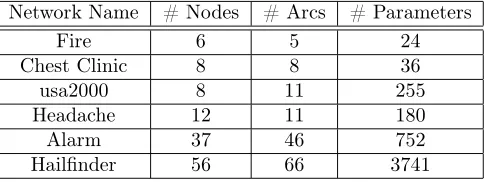
Table 2: Real networks used for evaluation.
Network Name # Nodes # Arcs # Parameters
Fire 6 5 24
Chest Clinic 8 8 36
usa2000 8 11 255
Headache 12 11 180
Alarm 37 46 752
Hailfinder 56 66 3741
• the “Weka” Java library for decision tree learning, in our implementation of Yang’s method [22]
7.3
Data
7.3.1 Causal Networks
We have selected two types of CNs for simulating data: real and artificial. The real networks are gathered from the Bayesian network literature and tools sam-ples. The Alarm and Hailfinder networks are from [23] and [24], respectively. Fire, Headache, Chest Clinic and usa2000 have been chosen from samples of Hugin GUI [25]. The artificial networks were created manually, with their structure and parameters chosen mostly randomly, but in such a way that a meaningful causal network is obtained. Networks were created with a varying number of variables, and all variables are discrete, as for the real networks.
Tables 1 and 2 show the nodes, edges, and parameters in each of the net-works. For each network, a single target attribute was chosen randomly and manually among the attributes near the end of the network.
7.3.2 Observational Data
Table 3: Number of records generated for each network
Network Name Number of Records
sample7 12800
sample15 20000
sample30 20000
sample45 20000
Fire 6400
Chest Clinic 2560
usa2000 11644
Headache 262144
Alarm 173328
Hailfinder 50000
7.3.3 Cost Data
We have randomly generated cost data for each data set. A randomly chosen subset of the attributes (20% of the total) was considered stable; these attributes are given a infinite cost.
Among the remaining 80%, some attributes were chosen to be semi-stable, in the sense that changing their value fromatoa′has a finite cost but the opposite
change has infinite cost (to simulate, for instance, attributes such as “experience level”, which can be increased through training but cannot be decreased). 5% of all cost values were set to infinity to model such semi-stable attributes. Other costs were chosen randomly from a uniform distribution between 0 and 10. pg
was set to 100 in all cases.
7.4
Results
We have experimented with both exhaustive and greedy search (ES, GS). Because ES is computationally prohibitive in large networks, we added a time threshold to this method, which varied from one to a few seconds per object, based on the size of network. When the threshold was exceeded, the best result until then was returned. The exhaustive search ran to completion in four datasets: Fire, ChestClinic, usa2000 and sample7.
For each network, we have repeated the following procedure 10 times (except for Hailfinder, where it was repeated only 5 times due to its computational cost): Generate random cost data for the network (according to the procedure explained above); randomly select 100 objects whereT 6=tg; use each method
to find the most profitable action for each object in the set; report for each method the averagennpobtained. These results were again averaged over the 10 (or 5) runs with different random costs. The final result is shown in Table 4.
Inspection of the table shows the following.
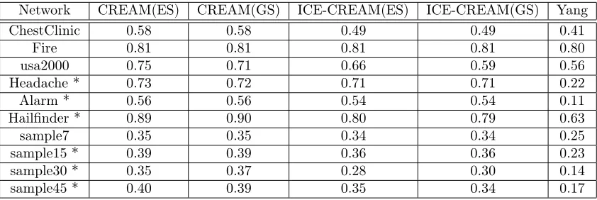
Table 4: Average normalized net profit obtained by CREAM, ICE-CREAM and Yang’s method on different networks. Asterisks indicate where ES was interrupted.
Network CREAM(ES) CREAM(GS) ICE-CREAM(ES) ICE-CREAM(GS) Yang
ChestClinic 0.58 0.58 0.49 0.49 0.41
Fire 0.81 0.81 0.81 0.81 0.80
usa2000 0.75 0.71 0.66 0.59 0.56
Headache * 0.73 0.72 0.71 0.71 0.22
Alarm * 0.56 0.56 0.54 0.54 0.11
Hailfinder * 0.89 0.90 0.80 0.79 0.63
sample7 0.35 0.35 0.34 0.34 0.25
sample15 * 0.39 0.39 0.36 0.36 0.23
sample30 * 0.35 0.37 0.28 0.30 0.14
sample45 * 0.40 0.39 0.35 0.34 0.17
good than for the informed CREAM method. However, the difference is often small. This suggests that ICE-CREAM can be used effectively in real-world problems.
2. ICE-CREAM outperforms Yang in each network. Again, this is not sur-prising, given that Yang implicitly relies on strong assumptions about causality, which seem unrealistic in practice, and are definitely invalid for the datasets used here.
3. Greedy search works well, in comparison to exhaustive search. On the four datasets where ES could be completed, GS obtained the same result in three datasets, and only slightly worse in the fourth (usa2000). This holds for CREAM as well as for ICE-CREAM.
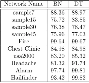
Table 5: Predictive accuracy of Bayesian networks and decision trees for the considered datasets.
Network Name BN DT sample7 88.36 88.97 sample15 75.72 83.85 sample30 76.38 78.47 sample45 75.96 77.03 Fire 99.64 99.67 Chest Clinic 84.98 84.98 usa2000 83.20 85.32 Headache 81.32 91.74 Alarm 97.74 99.81 Hailfinder 93.42 99.82
8
Conclusions and Future Work
In this paper, we have introduced the idea of using causal relationships in action mining, and argued why this should lead to better results. We have proposed a novel method called ICE-CREAM that first builds a causal network that indicates hypothesized causal relationships among the variables, then uses this causal network to recommend actions that can be taken to change the state of given objects into some goal state. Experiments show that ICE-CREAM leads to much higher gains than the best known current method for economical action mining, and confirm the expectation that this is due to the explicit use of causal relationships in ICE-CREAM.
While the proposed method is already a clear improvement upon the state of the art in action mining, it is still subject to improvement. Handling the uncertainty in the automatically induced causal network is currently the main bottleneck; the current method is computationally expensive and makes many assumptions that are known to be wrong. Recent results on efficiently comput-ing path probabilities in probabilistic graphs [26] could be exploited to improve this. Further, the current version of ICE-CREAM assumes there are no missing data, handles only discrete attributes, and assumes a binary target attribute.
Our current method is transductive: it does not return generally applicable action rules, but action set recommendations for concrete objects. A simple way to derive an action rule learner from it would be the following: predict action sets for a large number of objects, then use a standard rule learner to learn which actions are predicted under which circumstances.
In principle, the proposed method is not limited to economical applications, but could also be useful in, for instance, life sciences. It is to be expected, however, that as the complexity of the real causal relationships increases, the difference between approximate causal inference using an incomplete network and using no causal reasoning at all diminishes. It remains to be explored for what range of applications the method is practically useful.
Acknowledgements
Part of this research was carried out while the first author was on sabbatical leave from IUT and visiting KU Leuven. The authors thank Sander Beckers and Wannes Meert for proofreading and comments.
References
[1] Z. Ras and A. Wieczorkowska, “Action-rules: How to increase profit of a company,” Principles of Data Mining and Knowledge Discovery, pp. 75– 116, 2000.
[2] Q. Yang, J. Yin, C. Ling, and R. Pan, “Extracting actionable knowledge from decision trees,” Knowledge and Data Engineering, IEEE Transactions on, vol. 19, no. 1, pp. 43–56, 2007.
[3] Q. Yang, J. Yin, C. Ling, and T. Chen, “Postprocessing decision trees to extract actionable knowledge,” in Data Mining, 2003. ICDM 2003. Third IEEE International Conference on. IEEE, 2003, pp. 685–688.
[4] Z. Ras and L. Tsay, “Discovering extended action-rules (system dear),”
Intelligent Information Systems, pp. 293–300, 2003.
[5] L. Tsay and Z. Ras, “Action rules discovery: System dear2, method and experiments,”Journal of Experimental & Theoretical Artificial Intelligence, vol. 17, no. 1-2, pp. 119–128, 2005.
[6] ——, “Action rules discovery system dear_3,” Foundations of Intelligent Systems, pp. 483–492, 2006.
[7] J. Pearl, Causality: models, reasoning, and inference. Cambridge Univ Press, 2000, vol. 47.
[8] P. Spirtes, C. Glymour, and R. Scheines,Causation, prediction, and search. MIT press, 2001, vol. 81.
[10] G. Piatetsky-Shapiro and C. Matheus, “The interestingness of devia-tions,” in Proceedings of the AAAI-94 workshop on Knowledge Discovery in Databases, vol. 1, 1994, pp. 25–36.
[11] A. Silberschatz and A. Tuzhilin, “On subjective measures of interestingness in knowledge discovery,” in Proceedings of KDD-95: First International Conference on Knowledge Discovery and Data Mining, 1995, pp. 275–281.
[12] Z. Ras, E. Wyrzykowska, and H. Wasyluk, “Aras: Action rules discov-ery based on agglomerative strategy,” Mining Complex Data, pp. 196–208, 2008.
[13] K. Wang, Y. Jiang, and A. Tuzhilin, “Mining actionable patterns by role models,” in Data Engineering, 2006. ICDE’06. Proceedings of the 22nd International Conference on. IEEE, 2006, pp. 16–16.
[14] A. Tzacheva and Z. Ras, “Association action rules and action paths trig-gered by meta-actions,” in Granular Computing (GrC), 2010 IEEE Inter-national Conference on. IEEE, 2010, pp. 772–776.
[15] Z. He, X. Xu, S. Deng, and R. Ma, “Mining action rules from scratch,”
Expert Systems with Applications, vol. 29, no. 3, pp. 691–699, 2005.
[16] C. Silverstein, S. Brin, R. Motwani, and J. Ullman, “Scalable techniques for mining causal structures,” Data Mining and Knowledge Discovery, vol. 4, no. 2, pp. 163–192, 2000.
[17] A. Darwiche,Modeling and reasoning with Bayesian networks. Cambridge University Press, 2009, vol. 54, no. 2.
[18] D. Margaritis, “Learning bayesian network model structure from data,” DTIC Document, Tech. Rep., 2003.
[19] M. Scutari, “Learning bayesian networks with the bnlearn r package,”Arxiv preprint arXiv:0908.3817, 2009.
[20] ——, “bnlearn, bayesian network structure learning,” http://www.bnlearn.com/.
[21] decision system laboratory of Pittsburgh university, “Jsmile, java interface for smile,” http://genie.sis.pitt.edu/about.html.
[22] the university of Waikato, “Weka, data mining software in java,” http://www.cs.waikato.ac.nz/ml/weka/.
[23] I. Suermondt and R. Chavez, “The alarm monitoring system: A case study with two probabilistic inference techniques for belief networks.”
[25] “Hugin lite 7.5 samples,” http://www.hugin.com.