The computation of two dimensional manifold with angle self adaptive algorithm

(1)

Journal of Chemical and Pharmaceutical Research, 2014, 6(3):1382-1388

Research Article

_{CODEN(USA) : JCPRC5}

ISSN : 0975-7384

The computation of two-dimensional manifold with angle self-adaptive

algorithm

Meng Jia and Peng Yao

Department of Electrical Engineering, Xinxiang University, Xin Xiang, China

_____________________________________________________________________________________________

ABSTRACT

The paper described vertex combine theory, angle self-adaptive algorithm and the boundary judgment approach to compute two dimensional-manifold. The density of the flows originating from the local manifold is determined by the adaptive angle. For every flow the single step arc-length increasing is the same, and it is easy to calculate the distance between the adjacent flows. This method makes a step to study the three dimensional non-autonomous dynamical system.

Keywords: Non-linear System, Manifold, Chaos, Hindmarsh-Rose (HR) Neuron, Angle Self-adaptive

_____________________________________________________________________________________________

INTRODUCTION

HR model is derived from the Hodgkin-Huxley (HH) model. HR model can not only analog the electric potential of neurons’ discharging, but it can also simulate the frequency of neurons’ discharging. The model contains both a fast changing system and a slow changing system[1]. The coupling from circuit and synaptic leads to circadian rhythm changes of the two models. Under stimulation of the periodic signals, two neurons that have the same parameters and chaos situation can be synchronized with stimulation signals through phase cycle[2]. Under the constant current and the weak periodic signals, the HR neurons model has some characters of non-liner discharging[3]. The non-liner system can always be presented in the form of differential equations.

The computation of manifold plays an important role in analyzing the dynamical system. We can see both the stable and unstable trends form the visual manifold figures. The manifold can’t be solved from the differential equations directly[4], and it can only be solved through numerical analysis. The paper shows the affection of parameter selection to the non-liner system first; then it introduced how to compute the equilibria using the phase planes; throng the computation of the Jacobian matrix at equilibria and lining the non-liner system we can get the eigenvalues and eigenvectors respectively; at last after estimating the local manifold and analyze the errors of the approximation, we introduce two methods to compute the two-dimension unstable manifold of the HR model.

EXPERIMENTAL SECTION

The HR model equation can be showed as:

3 2

2

,

[ (

)

].

x

y

a x

b x

z

I

y

c

d x

y

z

r s x

δ

z

=

−

+

− +

= −

−

=

−

&

(2)

In the equation, x presents the electric potential of the membrane, y means the resume parameter and z stands for the slow changing currency[5].

2.1 The parameter selection of HR model

In term of HR model differential equation, the selection of parameter is very important to study and analyze the non-liner system. Because the HR is fast and slow changing system, when choosing certain parameters, the system may have chaos situation. Bifurcation is one of the circumstances when chaos happens. Before choosing the parameter, we can do some bifurcation analysis for each parameter to determine the proper parameters[6].

It is very hard to solve the analytical solution of the HR model differential equation, so we can approximate the equations (1) as

3 2 1

2 1

1

(

) ,

(

) ,

[ (

)

] .

k k

x

y

ax

bx

z

I dt

y

c dx

y dt

z

r s x

δ

z dt

+

= + −

+

− +

=

+ −

−

= +

− −

(2)

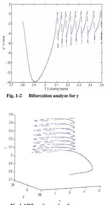
Using the Iteration method, we can have the numerical solution of the given initiation conditions. Taking parameter I as an example, when choosing a=1，b=3，c=1，d=5，s=4，r=0.006，

δ

=-1.6, dt =0.005 and I arranging from 2.8 to 3.5, we can do bifurcation analyzing for parameter x, y and z.

[image:2.595.140.490.397.750.2]

The bifurcation situation has been done under the following processing: when parameter I grows from 2.8 to 3.5 by 0.001 for each step, we iterate 50 times for each I. We record the result when the iteration number is over 20. Then we see how many periodic points the equation (2) has as I equal certain value. If it has only one periodic point, there will be one point on the figure at corresponding ‘I’ ’s coordinate. Otherwise there will be many points and the bifurcation happens.

Fig.1-1 Bifurcation analyze for x Fig. 1-2 Bifurcation analyze for y

[image:2.595.311.496.399.748.2]

(3)

The figure 1-1 presents that x has only one periodic point when parameter I changing from 2.8 to 3.1. But it began to have many periodic points when parameter I was at certain value such as I=3.12. In term of y, parameter I leads to the same results as figure 1-2 has shown; but seen form figure 1-3, z have a different results: when parameter I changing in the same interval, z always has one periodic points. Figure 1-4 shows two dimensional bifurcation of x and y when parameter I changing in interval [2.8，3.5]. As the three dimensional bifurcation showed, when I changing from 2.8 to 3.5 by 0.001 for each step, for most steps it was a point, but for some steps as I=3.2, it was a plane. It means that when I chosen certain value, the system has bifurcation situation. From the simulation results, we could also know that the fast changing parameters play more important role in bifurcation situation(x, y are fast changing parameters, z is slow changing parameter). In the same way, keeping I as a constant parameter, we can also do bifurcation analyzing to other parameters. In this paper we choose the parameter I=3.2.

2.2 Liner disposal to HR model

Before computing the manifold of non-liner system, we should liner the differential equation first. When the bifurcation analyzing has been done and the parameters have been decided as 2.1 showed above. The equilibria of the HR model system

S

₀ was （-0.7138，-1.5479，3.5446）. After lining HR model and computing Jacobian matrix we can get the eigenvalues

λ

=（-6.998，0.1669，0.0137）and the corresponding eigenvectors

1

V

=（0.6433， -0.1613，0.1386）；

2

V

=（-0.7656 ，-0.9867 ，0.9759）； 3

V

=（-0.0022 ，-0.0224 ，0.1686）. The HR model has two positive eigenvalues and one negative eigenvalue, so it contains a two dimensional unstable manifold and one dimensional stable manifold.

RESULTS

The local manifold approximation and contingent analyzing are very different. Local manifold approximation means estimating the local manifold as equilibria is the center, which also means estimating the initiated condition. The contingent analyzing which analyze the errors in manifold computing is to get the minimal errors.

3.1 The local manifold approximation of HR model

The unstable manifold can be defined as:

0 0

(

)

{

: lim

( )

}

u k

loc _k

W

S

x U

F

x

S

→−∞

= ∈

=

(3)

The local manifold approximation is very important to the globe manifold computing. If the local manifold is too small, it will slow down the computing speed. It will decrease the computing accuracy of manifold if the local manifold is too large[7].

In term of HR model, we can make the equilibria as the center and

r

₀

/

λ

₂， 0

/

3

r

λ

as the long axis and short axis respectively to determine an ellipse.(The scale of the ellipse can be adapted by

r

₀). The plane of the ellipse can be

fixed by the eigenvectors

V

₂

r

and

V

₃

r

[8].

3 2

0 0 0

2 3

(

)

V

sin( )

V

)

x S

S

r

θ

λ

=

+

r

( cos( )

(4)

We can also make

r

₀ as the radius and the equilibria as the center to determine a circle. The plane of the circle is also fixed by eigenvectors

V

₂

r

and

V

₃

r

.

0 0 0 2 3

(

)

sin( ) )

x S

=

S

+

r

θ

V

+

θ

V

r

( cos( )

(5)

3.2 Contingent analyzing

The surface of HR model’s three dimensional unstable manifold is composed by lots of triangles or trajectories. Taking the triangles as an example, we show how to determine the vertexes of the triangles to minimize the errors.

Assuming two vertexes of the triangle are known as

x

₁， 2

x

， we have to find the third one 3

(4)

3

( )

x

=

f

x

(6)

1 2 1 2

( )

(

)

f x

−

f x

≤

L x

−

x

(7)

x

is the points used to compute

x

₃ on the same trajectory but former ring. L is the Lipschitz constant of

f

。

1 2

( )

(

)

(

)

f x

=

a x

−

x

+

b x

−

x

(8)

Along the trajectory,

f x

( )

can be extended in its opposite tangent direction to intersect with line

x

₁

x

₂，the point of intersection

x

%

must satisfy：

1 1 2 2

1 2

x

β

β β

+

=

+

%

(9)

We can simple the principle as：when

x

%

is between 1

x

and

x

₂，it satisfy the minimal errors，which means it catches up with the up-wind condition. Only then can we add dot

x

₃ to the manifold surface. The plane determined by

x

₁

x

₂

x

₃is the contingent approximating of global manifold[5] [9] [10].

DISCUSSION

The global manifold comes from the local manifold basing on the property of invariant manifold. All trajectories composing the global manifold begin form the local manifold. To compute global manifold from local manifold the integral time and step arc-length should be set. The unstable manifold computing equation is as flowing:

0 0 0

0

(

)

{

: lim

( )

}

(

))

u n t t u

loc

t t

W

S

x

R

ϕ

x

S

ϕ

W

S

→−∞ ≥

= ∈

=

U

(10)

4.1 Self-adaptive theory for HR model unstable manifold computing

The self-adaptive method focuses on computing the trajectories to compose the global manifold. From angle

θ

=0 to

θ

=

2 π

, the self-adaptive parameter



θ

changes depending on the max distance of the adjacent trajectories. When the distance is beyond the threshold (



d <d

,



d

is the threshold of the distance，

d

stands for max distance of the adjacent trajectories), we will decrease



θ

depending on equation (11) to compute another trajectory. Otherwise if the distance below 0.1*



d

, we should increase



θ

. Only when distance is between [0.1*



d

,



d

], can we get the trajectory we needed and the compute angle

θ

=

θ

+



θ

. One thing should be taken care of is that: the distance between two adjacent trajectories will increase sharply when the bifurcation situation happen. Hereafter we set rough adaptive equation and fine adaptive equation for



θ

as (11).

2 d

d d

0.1 d

0.1 d <d

d

-

(d 10

d) d <d

3 d

lg (d

d) d>3

d

θ θ

θ

θ θ

θ

− × ÷

≤

×





_×

_≤



=



× ÷ ÷

≤ ×



_÷

_×





(11) Computing steps:

1) Determine the parameters using (2). And approximating the local manifold using (4);

(5)

3) Determine the total integrating steps, single step time and arc-length for each step. The more the total steps are, the more details will be shown on global manifold surface.

4) Based on (10) (11), we compute the trajectories and change the angle



θ

to increase

θ

.

5) Repeat the step 4 unless

θ

>

2 π

.

Simulation and results analyzing:

Under the condition a=1，b=3，c=1，d=5，s=4，r=0.006，

δ

=-1.6, I=3.2. The distance threshold is 0.3 and the changing arrangement is

10

−2

−

10

−20. We set the total steps as 150 and single step arc-length as 0.05. We got the following figures:

Fig. 2-1 Self-adaptive parameter manifold Fig. 2-2 Local manifold and trajectories

Fig. 2-1 presents the global manifold including the trend and density of all trajectories. Fig. 2-2 shows the local manifold and the starting ellipse of all trajectories. We can see most of the trajectories starting from a small angle because it has bifurcation situation then and the distance between two adjacent trajectories increasing sharply. Only by decreasing the shelf-adaptive parameter can the accuracy be improved.

The computing errors for self-adaptive method can be measured by equation (12):

( ) 1

(

)

i

f

ε

= Σ

ε

(12)

1

ε

means the approximating errors of the local manifold and

f

( )i

( )

ε

₁ refers to

ε

₁ has been integrated by ‘i’ times.

ε

stands for the total errors.

4.2 Angle constraint theory for HR model unstable manifold computing

The angle constraint method[12] computes manifold through increasing the number of rings. Hence the max distance

d

between two adjacent rings and the distance of the adjacent dots in the same ring should be set. If the dots are too far from each or it didn’t satisfy up-wind condition, a new dot should be added between them and we also need rules to judge this. There were already some methods to do so [13]. But the unique methods in this paper are: First we don’t drop the dots which have always been computed even it doesn’t match the criteria. Because they are dots of the manifold and what should be done is interpolating new dots rather than replacing them; second, we interpolate dots in the former rings to compute news ones in the current ring rather than interpolate dots in the current ring directly. Such as:

If

x x

_ij *

>

d

,

x

*

=

f x

(

_{( 1)(}_i₋ _j₊₁₎

)

,

x

*refer to the dot should be replaced in some methods;

We add new dots: 1 ( 1) 2 ( 1)( 1) 1 2

(

i j i j

)

new

x

f

β

β β

−

+

− +

=

[image:5.595.188.494.218.401.2]

(6)

Only when

x x

_ij _new

<

d

and

x x

* _new

<

d

;

We treat

x

_new as

x

_{i j}₍ ₊₁₎ and

x

*as

x

_{i j}₍ ₊₂₎.

Computing steps:

1）Determine the parameters using (2), and approximating the local manifold using (5).

2) Determine the minimal and max value of the constraint angle. We should also certain the distance between two adjacent rings and the max distance of the two adjacent dots on the same ring. Beside we need the total rings’ number.

3) We compute the distance using angle constraint method to determine if it needs to add new dot, (When adding new dots, we use the unique methods)

4) Repeat step 3, when all dots on the ring satisfy the rule, we will begin the next ring and the computing is over when the total ring satisfy the rule.

Simulation and results analyzing:

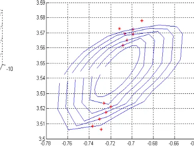
[image:6.595.126.300.314.474.2] [image:6.595.290.480.322.469.2]

We set the max angle as 0.1 and the minimal angle as 0.0025. The max distance between two adjacent rings and the distance of the two adjacent dots on the same ring are both 0.05; the total ring numbers are 150. The results are as the following:

Fig. 3-1 Angle-constraint manifold Fig. 3-2 Increasing loops and adding dots

Because the angle constraint method saves unnecessary dots around the local manifold to control the numbers of the dots on manifold surface, it saves the computing time but decreases the accuracy. Fig.3-1 shows the global manifold and Fig. 3-2 shows the local manifold and the increasing numbers of dots (”*” stands for the new adding dots).

The computing errors for angle constraint method can be measured by equation (13):

( ) 1

(

)

i new

x

f

δ

= ΣΣ −

+ Σ

ε

(13)

new

x

ΣΣ −

are the total interpolation errors and

Σ

f

( )i

( )

ε

₁ are the whole integration errors.

CONCLUSION

The paper introduced HR model and analyzed parameters bifurcation of the differential equation to show: the selection of parameters of the equation will cause the bifurcation situation even chaos circumstance. HR is a fast and slow system and the fast changing parameter is the main force for bifurcation. Beside, the article also described the local manifold approximation and contingent analyzing, which determined the computing speed and accuracy.

(7)

Acknowledgement

The work is supported by Tackle Key Problems in Science and Technology of He Nan province in China (Grant No.112102210014), Tackle Key Problems in Science and Technology of Xinxiang city in China (Grant No.ZG11009).

REFERENCES

[1] Q P Hu, Y Q Ren . Journal of WuHan University of Science and Engineering，2008，21（9）：19-24 [2] J Wu , JX Xu, DH He , Jin W. Acta Physica Sinica, 2005, 54 (7)：3457-463

[3] R Huerta , M I Rabinovich . Physics Letters: A, 1999, 264(10):289-296 [4] Michal Branicki , Stephen Wiggins. Physica D 238, 2009, Page(s) 1625–1657. [5] G H Zhang . Tong Ji university, 2007.3: 50-53

[6] Q C Zhang . Tian jin university publication， 2005.1：37-45 [7] M Dellnitz , A Hobmann . Num. Math, 1997, 75:293-317.

[8] B Krauskopf , H MOsinga. Appl. Dyn. Sys, 2003, 2(4):546–569.

[9] B Krauskopf , H M Osinga , Doedel E J, et al. Bifur.Chaos.Appl.Sci.Engrg, 2005, 15(3):763–791. [10] J Guckenheimer , A Vladimirsky . Appl. Dyn. Sys, 2004, 3(3): 232–260.

[11] M E Henderson . Appl. Dyn. Sys, 2005, 4(4):832–882.