Recursive Gauss Newton based training algorithm for neural network modelling of an unmanned rotorcraft dynamics

(1)

56 Int. J. Intelligent Systems Technologies and Applications, Vol. 13, Nos. 1/2, 2014

Recursive Gauss-Newton based

for

neural network modelling of

rotorcraft dynamics

training

algorithm

an

unmanned

Syariful S. Shamsudin

Department of Aeronautical Engineering,

Faculty of Mechanical and Manufacturing Engineering, Universiti Tun Hussein Onn Malaysia,

86400 Parit Raja, Batu Pahat, Johor, Malaysia E-mail: [email protected]

XiaoQi Chen*

Mechanical Engineering Department, University of Canterbury,

Christchurch 8041, New Zealand Telephone: +64 3 3642987 ext. 7221 Fax: +64 3 364 2078

E-mail: [email protected] *Corresponding _author

Abstract: The ability to model the time varying dynamics of an unmanned rotorcraft is an important aspect in the development of adaptive flight controller. This paper presents a recursive Gauss-Newton based training algorithm to model the attitude dynamics of a small scale rotorcraft based unmanned aerial system using the neural network (NN) modelling approach.

It

focuses on selection

of optimised network for recursive algorithm that offers good generalisation performance with the aid of the cross validation method proposed. The recursive method is then compared with the off'-line Levenberg-Marquardt (LM) training method to evaluate the generalisation performance and adaptability ofthe model. The results indicate that the recursive Gauss-Newton (rGN) method gives slightly lower generalisation perfbrmance compared with its off-line counterpart but adapts well to the dynamic changes that occur during flight. The proposed recursive algorithm was found effective in representing helicopter dynamics with acceptable accuracy within the available computational time constraint. Keywords: Artificial neural network; system identification; rotorcraft dynamics; unmanned aerial system; recursive Gauss-Newton.

Reference to this paper should be made as follows: Shamsudin, S.S. and Chen, X.Q. (2014) 'Recursive Gauss-Newton based training algorithm for neural network modelling of an unmanned rotorcraft dynamics', Int. J. Intelligent

Systems Technologie,r and Applications, Vol. 13, Nos. 1/2, pp.56-80.

Biographical notes: S.S. Shamsudin received the BEng (Hons.) in Aeronautical Engineering and MEng in Mechanical Engineering from the Universiti Teknologi

(2)

rGN based training algorithmfor neural netvvork modelling

Malaysia, Skudai, Johor, Malaysia, in 2003 and 2007, respectively. He is currently a PhD candidate at the Mechanical Engineering Department, University of Canterbury, Christchurch, New Zealand. His current research interests include aircraft and rotorcraft system identification, intelligent adaptive control and unmanned aerial system design.

X.Q. Chen received the BE from South China University

of

Technology, Guangzhou, China,

in

1984, the MSc from Brunel University, Uxbridge, UK,

in

1986, and the PhD from the University of Liverpool, Livelpool, UK, in

1989. He is currently a Professor with the Mechanical Engineering Department, University ofCanterbury, Christchurch, New Zealand. Research interests include: mobile robots including unmanned aerial vehicle, unmanned underwater vehicle, GPS-guided autonomous land vehicle, walking machines and climbing robot; human-robot collaborative systemi resources and environmental measurement, monitoring, management and control; assistive device for rehabilitation; machine health monitoring, diagnosis and prognosis; vibration-based energy harvesting for wireless instrumentation; manufacturing process automation; machine vision; bio-instrumentation and control; precision measurement and inspection; 3D printing of bio-scaffolds. He received the Singapore National Technology Award in 1999. He was a recipient of China-UK Technical Cooperation Award. This paper is a revised and expanded version of a paper entitled 'Recursive Gauss-Newton Based Training Algorithm for Neural Network Modelling of an Unmanned Helicopter Dynamics' presented at l9th International Conference on Mechntronics and Machine Vision In Practice - Il[ ' V1P, Auckland, New Zealand, 28-30 November. 2012.

1 Introduction

Rotorcraft based unmanned aerial systems (RUAS) are a commonly used platform of

unmanned aerial vehicles (UAV) and this platform configuration have been widely used in numerous applications ranging from surveillance to safe and rescue operation. The rotorcraft or helicopter platform possesses the unique manoeuvring capabilities that can hover above

or near targets, which make

it

more suitable than fixed wing aircraft for high building structural inspection. Research efforts had been directed in this field to enable the UAV to execute these application autonomously which subsequently could eliminate accident risks to human pilots and increase higher chances of successful mission implementation.

(3)

58

S.S. Shamsudin and X.Q. Chen

approaches with successful implementation in real flight tests (Kendoul, 2012). However, the capability of the RUAS automatic ffight controller can be further improved with the development of self tunable and flexible controllers such as the NN based flight controller that can be deployed and integrated into different rotorcraft platforms in shorter development time. Another benefit ofNN based controller includes the ability to adapt to platform changes such as payload, sensors or changes in the dynamic system.

In recent development of real-time adaptive control system, the NN approach has found growing success in the development of automatic flight control system due to their ability to leam complex mapping from the flight data. This would make the representation of the system dynamics much more straight forward, whereas the complex mathematical model is much more difficult to develop. The NN calculation is parallel in nature, which leads to faster calculation speed in an intensive computation problems (Balakrishnan and Weil, 1996). Furthermore, the NN has the ability to adapt well to a changing environment which makes

it

suitable for adaptive control application. Typical NN based control schemes can be categorised into six main classes as follows (Norgaard, 2000):

a

direct inverse controller internal model controller (IMC)

feed-forward controller with inverse model feedback linearisation controller

optimal controller

NN based model predictive controller (NNMPC).

Samal (2009), Norgaard (2000) and Agarwal (1997) suggested that the first five types

ofNN

controller schemes fall under direct adaptive control class where the NN is used to update the controller parameters. Whereas, the NMPC is an indirect type of adaptive controller where the NN model is used to aid the existing conventional MPC controller to achieve the desired reference trajectory. Figure

I

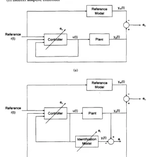
shows the basic configuration structure of the direct and indirect adaptive control system for a dynamic system. In direct adaptive controllers, the control parameters are updated directly to minimise the tracking error. The calculation

of the controller parameters or gains does not rely on the dynamic system to update the controller parameters. Whereas in the indirect adaptive control configuration, a dynamic model is used to predict the response of the dynamic plant. The prediction from the dynamic model is assumed to be identical to the actual response and this information is used to minimise the tracking error of the system.

The non-linear and high order dynamics behaviour of a rotorcraft is typically hard to model using first principle modelling approach (direct physical understanding of forces and moments balance

of

the vehicle), and such approach can be inaccurate (Budiyono

et

al.,

2N9).

Dynamic model obtained using the

frst

principle approacb depends on many parameters which needs to be carefully identified through direct measurements of

geometrical or structural data. For aerodynamic parameters estimation, detailed experiment needs to be performed using wind tunnel facilities. The principle modelling approach requires considerable amount of theoretical knowledge and experiences about the rotorqaft

flight

and potentially would not produce

a highly

accurate results unless performed

(4)

[image:4.592.130.420.170.482.2]

rGN based training algorithm

_for

neural network

modelling

59 dynamic behaviours is unsatisfactory because ofthe accumulated uncertainty and modelling simplification (Mettler, 20031 Kendoul, 2012).

Figure

1

The configuration of adaptive conroi system: (a) direct adaptive controller and (b) indirect adaptive conffoller

Since the helicopter dynamics is nonlinear, the NN based system identification approach using the NNARX (Neural Network-Auto Regressive structure with eXtra inputs) model structure can be used

to

address such

a

problem. Here, the linear model structure such as

ARX

model structure was introduced as the basic

NN

model structure while

static feed-forward multi-layered perceptron

(MLP)

network was used

to

introduce non-linearity

into

the model estimation. Similar

to

stability features

of ARX

model structure, the prediction

from

the

NNARX

model was considered stable since there

(5)

60

and Chen (2012) where the findings exhibit the capability ofneural network approach and its effectiveness in modelling the dynamic response accurately using second order method such as the Levenberg-Marquardt (LM) method.

Although the NN

is

superior

in

terms

of it

prediction accuracy, the dynamic model identified from NN can be inaccurate due to many problems such as incorrect model structure

selection, incorrect input vectors selection and over-fitting due to the excessive number

of

neurons. Previous attempts to model the non-linear unmanned helicopter dynamics using the off-line NN modelling has successfully modelled the dynamics of the helicopter, resulting in low mean or standard deviation of the residual values (Samal, 2009; Putro et al., 2009). However, past efforts in identifying the helicopter dynamics did not include the effect

of

embedded memory or model order of the NNARX networks on generalisation performance for the modelling problem considered. The validation methods introduced in this work can be used to ensure that the NNARX model fits well with observations and aid the neural network modeller to select the optimised network structure for prediction with an acceptable accufacy.

Furthermore, most NN based modelling techniques attempt to model the time varying dynamics of an UAS helicopter system using

offline

modelling approach. The model which is generated and trained once from previously collected data is not able to represent the entire operating points of the flight envelope very well (Samal, 2009). Several attempts such as Samal (2009), Samal et al. (2008, 2009) were made to update the NN prediction model during flightusing mini-batch LM training (LM training with small numberof data samples). However due to a limited amount of processing power available in the real-time processor, such methods can only be employed to relatively small networks and they are limited to model uncoupled helicopter dynamics. In order to accommodate the time-varying properties of helicopter dynamics which changes frequently during flight, a recursive based learning algorithm is required to properly track the dynamics of the system under consideration. Furthermore, the usage of recursive algorithms such as recursive Gauss-Newton (rGN) or recursive Levenberg-Marquardt (rLM) reduces the computation complexity of the off-line training method without having to invert the

full

Hessian matrix in every iteration (Ngia and Sjoberg, 2000).

The present study is concemed with the modelling and identification of a helicopter based UAS. The multiJayer perceptron (MLP) network architecture is considered for this purpose and different network structures are compared and analysed

to

determine the optimised network structure, with good generalisation performance using the aid of the cross validation method proposed. Based on the network structure selection, a recursive prediction error algorithm such as the recursive Gauss-Newton method is proposed to train the neural network model. The generalisation and adaptability performance of the recursive algorithm is then compared with the off-line algorithm to verify

if

the prediction quality has improved over its off-line counterpart.

2 Platform

description

The UAV platform which was used in this research is a conventional electric model helicopter

(6)

_for

neural network

modelling

6l

[image:6.594.150.376.221.364.2] [image:6.594.101.429.396.476.2]

responses. Furthermore, TREX600 was also equipped with a high efficiency high torque brushless motor that allows the helicopter to carry about 2 kg payloads with an operation time of about 15 m. The basic UAV platform shown in Figure 2 had been modified to make room for installing necessary electronic equipments which gathers flight data for dynamic modelling and control system design. Some key physical parameters

of

TREX600 RC helicopter are given in Table 1.

Figure

2

The TREX600 helicopter used in the system identification experiment with

instrumentation equipment fitted between fuselage and landing gear (see online version lbr colours)

Tabte

I

The specification of the TREX600 ESP helicopter

Spetifications TREX6OO ESP

Length Height

Main Rotor Diameter Tail Rotor Diameter Weight

Endurance

l.16 m 0.4 m 1.35 kg 0.24 m 3.3 kg

l-5 min

3 Collection

of

flight

data

The flight test was conducted on the UAV helicopter platform in calm weather conditions. Different flight manoeuvres were conducted to excite the desired dynamic of interest. For example, after the helicopter reached steady and level condition, the yaw dynamics was excited using only tail collective pitch command while other input commands were used to balance the helicopter in such a way to make the vehicle oscillate roughly around the operating point of interest.

Training and validation data were collected from specifically designed frequency swept excitation signal suggested in Tischler and Remple (2006). This type of signal is commonly used to collect experimental flight data

in

aircraft and rotorcraft system identification.

(7)

62 It

is recommended that the pilot executes two good low frequency cycle inputs (20 s) and then gradually increase the swept frequency to mid and higher frequencies before ending the manoeuvre in the trim position. Starting and ending the record

in

aircraft trim state enables concatenating flight data collected from several test runs while at the same time ensuring rich signal content.

All

measurements of the helicopter's state variables were collected using an inertial measurement unit (IMU) where the data that were recorded during test were Euler angles:

roll

_/,

pitch 0 and yaw V; angular rates in body coordinate frame: roll rate, p, pitch rate, q and yaw rate,

r

and body accelerations: o", ao, a".The control inputs measured during the experiment were the stick deflection from the pilot's collective pitch 6,,,1, pedal 57,ea,

longitudinal cyclic 56n and lateral cyclic d1o1. The four servomotor signals

":

lsette

sAUx sELE

"rrof'

.

can be translated to pilot's stick positions (Input range ₌

*1),

6

:

_{l6u.6Lot 6"ot}

5r.o)'

,

by means of a linear transformation:

6

:

A-r

("

_{- tr,o^)}

(1)

where .s1,;,, are the servo signals at trim values which indicate the necessary pulse width values to level the swash plate position. Matrix ,4 (mixing gains) has to be determined through the measurement

of

servo signals

for

different stick positions to get the exact relationship between pulse width commands sent to the servos and the requested control inputs.

The common frequency range

for

the excitation signal used

in

rotorcraft system identification and control are between 0.3-20 rad/s. It is also recommended in Tischler and Remple (2006) that an identical filter should be used for all output and input signals with a cut-off frequency 5 times higher than the maximum excitation signal frequency. Hence to reduce the noise in sensors data, the

curoff

frequency of the low pass filter used in this study was selected at

l5

Hz. The sampling rate of the sensors was selected at 100 Hz which was at least 25 times higher than the maximum excitation frequency.

4 Neural network model

structure

(8)

_for

neural network

modelling

63 The NN input-output relationship of a dynamic system described in this research was adapted from standard ARX (Autoregressive structure with extra inputs) model structure as

in Ljung ( 1999). In a NN based ARX (NNARX) model structure, the variable to be estimated and other influencing variables including their time lags are typically fed into a static feed-forward network such as multi-layer perceptron (MLP) network (Samarasinghe, 2007). The

conceptual diagram of NNARX model structure used to identify the non-linear relationship of helicopter's attitude dynamics is shown in Figure 3. Note that the regression vector or inputs vector to the network is typically chosen to include ny past output measurement data and

n,

past input data. The number of past output and input data to be fed to the network is left for user choice.

Figure

3

The NNARX model structure with preselected regression vectors (see online version for colours)

Output Layer

Hidden Layer

lnput I Input 2

The fully connected MLP network architecture containing only one hidden layer, was chosen to leam the nonlinear relationship of the NNARX model. The output calculation from the

MLP structure to represent the NNARX predictor is given as follows:

'i

(tlo)

:

hi

(p, o)

(i,r,^,,(i,^,,,

_*

u,)

\fi

"\Fi

I

-D

- ri

*

br)

/

with,

h

:

I,2,3.-.

H

i,:1,2,3...n

(2)

(9)

64

and the parameter and regression vectors are given by:

0

:

_l*ni

Wn

bI b2]

e Q)

:

lP''

Pr

" '

q,,]

:

fu(t),y(t

-

r),

"',aft -

n),

t\t),u(t-

1),..

.,rt(t

- n)]

where tr.r6; is the weights matrix between the input layer and the hidden layer and

I4l;'

is the weights matrix between the hidden layer and the output layer. The functions

_f

_{iQ") and}

f;(*)

are non-linear activation function for neurons in each hidden and output layers. The

symbol 11 denotes the number ofneurons in the hidden layer while bL and,b2 are the bias elements for the input layer and output layer. The number of inputs and outputs ofthe neural network are presented by rn. and n respectively.

5

Cross

validation method

The choice

of

higher number

of

past output and input

will

results

in

a larger network architecture that

will

have a lower MSE but poor generalisation ability (Billings et al., 1992). This means that the network model predicts the estimation data set (training set) with

great accuracy but fails to represent a new data that was not used in the training process. Large assignment of hidden neurons also contributes to poor generalisation performance (Wilamowski, 2009).

Cross validation is a statistical method that is normally used in data mining problems to determine the model sffucture selection and to compare generalisation performance of

different learning methods. The simplest method to conduct validation analysis is to use the hold-out method where the measurement data is divided into training and test sets with user defined split ratio. Subsequently, the training set is used for model training and the test set data for error rate estimation of the trained model. However, the downside of this method is that the model evaluation can produces a high variance error. Depending on how the split ratio is defined, the prediction error evaluation may be inconsistent for different partitions of data that forms the training and test sets (Kohavi, I 995).

To overcome this problem and utilising the available overall data, the k-fbld cross-validation method was used to reduce the variance by averaging error over & data segments. Kohavi (1995) suggested that cross validation

with

10-20 folds would gives reasonable estimate with low bias and variance error. In this method, the measurement data

N

is split

into

k

approximately equal

M

size data segments. Then, the training and validation are performed for /c-iterations where within each iteration, a single portion of the data segment at a certain index location shown in Figure 4

will

be used for validation after the training

of the remaining k

_-

1 data segments are completed. For each validation, the prediction MSE is calculated for the specific segment. The MSEs from each validation segment are averaged and combined together at the end of the iteration process using percentage root mean square error (% RMSE) as follows:

(3)

RMSE:

r-t r/2

-l

x100

I

N

KIVI

tf:,

Dlj,

(gt(t)

_-

_at(t))

(4)

(10)

rGN based training algorithmfor neural network

modelling

65 where

_9;(t)

denoted the predicted

NN

model output from a specific /c-validation data segment,

y;(l)

indicated the k-validation data segment and

y(t)

is the mean value of the measurement data.

Figure

4

The procedure of ft-fold cross-validation for A

:

5 (see online version for colours)

k=2

rtl

I

TI

-NOVh oooo@ uilud{ ooooo a0qoa

k:3

_I"-,I

k=4

_l-vl

k=5

_I".

Training

Validation

6

System

identification

methods

The system identification

for

inferring the helicopter dynamic model can be conducted using off-line (batch) and recursive based system identification methods. The estimation of a dynamic model in the off-line NN identification method involves the training process being canied out over some finite data gathered beforehand. Over the whole length of the data record, we determine the best weights (parameters vector 0) that give the best fit for

the measurement data over repetitive iterations. Obviously, the off-line methods have a disadvantage such as

it

is unsuitable for tracking time varying dynamics, as the amount

of computation time for the training phase

in

each iteration might exceed the available processing time (Norgaard,2000). The adaptive control is an example where a model needs

to be identified at the same time as a control law is calculated to compensate the time varying control variables. Even though the off-line training methods are not suitable for

(11)

66

To overcome the disadvantages of the off-line training methods, the recursive based system identification methods can be used in tracking time varying dynamics. The recursive model estimation

is

a system identification technique that enables us to infer a model that adapts to time-varying dynamics based on real-time data coming from the system. In contrast to off-line training method, the recursive methods enforce update to NN parameter vector based only on a single data at current sample t. To achieve real-time implementation

of

the neural network based system identification, the estimation

of

neural network's parameter vector d can be carried out using recursive algorithms as described in Billings

et

al. (1992), Norgaard (2000), Youmin and

Li

(1999), Ljung and Soderstrom (1983)' The recursive identification algorithms have several advantages over the batch methods. The implementation of the method is simpler, less memory-consuming with faster convergence since the redundancy in the data set is effectively utilised (Norgaard, 2000).

Recursive algorithm can also be implemented similar to the

offline

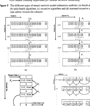
training where the recursive training is repeated several time on the finite training set Z N , collected in advance (Norgaard, 2000; Billings et al., 1991, 1992). Figure 5 shows the difference between the batch algorithm, mini-batch algorithm, on-line recursive algorithm and repeated recursive algorithm. The parameter vector

d

updating process usually start

with initial

random weights and

it

is carried out forward to the next iteration as computation progress. The implementation of batch and mini-batch algorithm is similar but differs in the number of data samples used for training. In the recursive algorithm methods, the parameter vector update is obtained in real-time as the measurement data become available from the instrumentation system. Figure 5(d) shows the implementation of recursive algorithm as an

offline

method. The parameter vector 0 is updated at each time sample

t

over a fixed data sample. At the end of first iteration, the last parameter vector d is used as the initial update to the second iteration step. This iteration process

will

stopped

ifthe

mean square criterion converges to pre-defined threshold as in batch training algorithm implementation.

6.1

Off-Iine system

identificationwith

neural network

After selecting the model structure, the next step in the system identification process is to determine the best weights (vector parameters d) that give the best fit between the NNARX

model and measurement data. This is achieved by minimisation

of

error cost function. As mentioned in Norgaard (2000), the measurement of prediction's closeness to the true outputs of the system is given by mean square elror (MSE) type criterion:

,

1rt

v11(g,z1y.):

_{*Dla@-a(le)1',}

(5)

t:1

with linear approximation of prediction error given by:

e(t,0)=a(t)-0(tl0)

(6)

(12)

[image:12.594.110.412.103.457.2]

rGN based training algorithmfor neural netvvork

modelling

67 Figure

5

The different types of neural network model estimation methods: (a) batch algorithm;

(b) mini-batch algorithm; (c) recursive algorithm and (d) repeated recursive algorithm

(see online version for colours)

Sreh No

i.t

:

I

EEEAEENEEEEE

E

t. lt.ttl c

d fr,rl

p

EEEEEEEENEEE

E

t "11'rt\ o

e'e,tl

0

EEEEEEEEEAEE

E

t' l['rl .

A

NEEOEEEEEEAE

E

t. tr. ill r

t t tt

0,,

trtrtrtrE]

tr

t . lP.;il (;

trtrtrtrtr

tr

| , lR,itl c

0.

trtrEtrtr

tr

I lR-itl i

0

trtrtrtrtr

tr

t -1e,il\ L

In

order to minimise the cost function

in

equation (5), the Levenberg-Marquardt (LM) iterative search algorithm was used for the neural network training process. The optimisation process

is

carried out iteratively over a given data set

to

achieve the minimum error criterion. The

LM

optimisation algorithm uses the Gauss-Newton Gradient

G(d)

and Hessian E(d) matrices, which were derived specifically for the neural network model in Yu and Wilamowski (2011), Ngia and Sjoberg (2000) and Norgaard (2000). These important matrices are represented in the following equations:

lJl

G(0):

_{*> ,v(tl0)le(t,0)l}

(7)

t\t 4

- t:7

R (o)

:

*

f

,ll _elo)_bt)

(tlo)f

(s)

NL''' t:l

where

t!(tl|)

is the Jacobian matrix that represent the first derivative of the one-step ahead prediction with respect to parameters vector 0. The procedure to calculate

matix

l!(tl9)

is

(13)

68

given in detailed in Yu and Wilamowski (2011) and Norgaard (2000). The Hessian matrix

R(d) has a dimension of d

x

d and Gradient vector G(0) with dimension of d

x

1, where d is the total number of elements (weights + biases) in the parameter vector d.

We could find the minimum of the error criterion by iteratively solving the following

equations:

g(t+l)-6Q.)ay()

ln

(ot,';

+

r(o)1] yter

:

-c

(oto)

(e)

(10)

where

_/(t)

is the search direction vector,

l

is the identity matrix and A(t) is a damping factor used for deciding the step size. In order to determine

),

the indirect method used in Norgaard (2000) is adopted by calculating the following ratio to determine the accuracy of

approximation:

(11)

eduction approximation

The main purpose of introducing the ratio calculation is to measure how well the reduction

of the criterion V1,1(0,

Zy)

matches the reduction predicted

by

approximation terms in denominator

of

ratio calculation

in

equation (11). The damping factor

l

is

adjusted accordingly

to

the ratio

r(t) by

some factor (Norgaard, 2000). The procedure

of

the

LM

algorithm with indirect method to determine

,\

is given

in

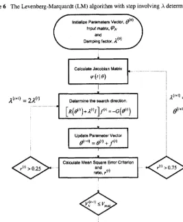
Figure 6. The reduction approximation (denominator term in equation (11)) is most likely a close approximation to error criterion Vy (0, Z

y),

if

the ratio

r{t)

value is close to one and parameter

)

should be reduced by some factor. However,

if

the ratio r'(t) is small or a negative value, parameter

)

should be increased. Additional stopping criterions are normally introduced to this algorithm to prevent minimisation problems or to force early stopping such as stopping criteria based on maximum number of iterations, sum of square error that drops below a certain threshold, upper bound for gradient and maximum weight change, maximum value of parameter ,\ or early stopping criterion due to training time constraint.

6.2

Recursive system identification with neural network

Recursive model estimation is a system identification technique that enables us to infer a model that adapts to time-varying dynamics based on real-time datacoming from the system. To achieve real-time implementation of NN based system identification, the estimation of

neural network's parameter vector 0 can be carried out using recursive algorithms such as

described in Billings et al. (1992) and Youmin and

Li

(1999). Batch method described in the previous section is deemed unsuitable for tracking time varying dynamic as the amount

of computation time

for

the training phase

in

each iteration might exceed the available processing time (Norgaard, 2000).

The recursive system identification method builds a model of the system at the same time as the measurement data is collected. The model is then updated at each time step, as

(14)

for

neural network modelling

recursive Gauss-Newton (rGN) method. For every data sample, the parameter vector d(f )

is updated by the recursive algorithm using the following equations:

69

e(t):

a(t)

-0(t)

R(t)

:

R(t

_-

r)

+'y(t)1,/,

(t)rr-'

_{ft)',p' (t)}

_-

n(l

-

1)l

A

til

:

A

(t

-

1.)

+

1,G)

R-t

Q),1'(t)

i-t

1t1e 1t1

(12) (13) (14)

where ,R(t) is an approximation of Gauss-Newton Hessian matrix, dt is the estimation of

pilameter vector of the NN model.

A-r (i;

is the weighting matrix and

1(/)

is the gain sequence at the current time step f . The simplest choice of weighting matrix

A-r

(l)

is an identity matrix as suggested by Billings et al. (1992). The forgetting factor

)(f

_{) is defined}

as a constant scalar variable which accounts for the amount of past data information to be included

in

the error criterion function.

If

the forgetting factor

is

I(t)

<

1, the term would make the estimation more adaptable to changes and sensitive to noise. Whereas,

if

[image:14.593.129.397.330.654.2]

I(r)

-+

1 as time increases, more old data are included in the criterion and the adaptation would fluctuate less during the learning process (Youmin and

Li,

1999).

Figure

6

The Levenberg-Marquardt (LM) algorithm with step involving ^

determination

lnitialize Parametes V*tor, B(o) tnput matnx, Qtt

ano Damping factor, 2(o)

1(i+tl _ 27(r)

r {rl

.1,+ll A' ' A'

'=-t

o(i+tl

-

0o Calculate Jacobian Matrix

v(tlo)

ln(d")+,r(4r]l(') =

-c(di,)

Calculate lrean Squae Error Crllerlon and

(15)

70

In practice, equations (12)-(14) are not calculated straightforward with inversion of matrix

/i-

1 _{(r) which}_requires_{computational complexity}_{of O(d3}

) (Ngia and Sjoberg, 2000). Ljung and Soderstrom (1983) had shown that using marix inversion theorem, the generalised rGN algorithm is rewritten to avoid full Hessian matrix inversion as follows:

p (t)

:

_lp

(t

_-

1)

_-

L(t)

s*'

(r)

Lr

(il)

_l^(t)

s(r)

:

1!r

(q

P _Q

_-

t)

_t:(r)

+

^

(r)

^(t)

L

(t)

:

P (r

_-

1) ₄₎

(t)

S-1 (t)

0(q:A(r-1)+

L(t)e(t)

(ls)

(16) (17) (18)

Note that the inversion of matrix

R-'(t)

had been reduced from

full

inversion of d

x

d matrix to S - I ( t ₎with

n

x

n dimension . Note that n denotes the number of outputs predicted in the model.

Equations (15)-(18) indicates that initial value of

P(0)

(d

x

d matrix) and parameter

vector

d(0)

need to be supplied

by

user at the beginning

of

the iteration. The initial

parameter

n".tot

d10; is usually selected as random values or pre-determined weights resulting from the off-line training. A common choice for P(0) is

P(0)

:

pI

with p being a large positive number (i.e., 102

-+

104) indicating little confidence in A1O;. This would cause the estimation to rapidly increase in the transient phase for a short period of time

dl

(Ljung and Soderstrom, 1983). As the estimation of parameters are quite poor at the beginning of the iteration, a lower forgetting factor should be selected at the initial stage for rapid adaptation and approaching unity as the time increases. The following strategies introduced by Ljung and Soderstrom (1983) is used for updating the forgetting factor term:

)(l):)")(t-1)+(1-)")

(1e)

where .\n and

)(0)

are design variables. The typical values of )o is 0.99 and .\(0) is in the rangeof 0.95

< )(0) <

1.

According to Ljung and Soderstrom (1983), the recursion ofequation (15) is numerically unstable due to round-off errors which build up and influence

P(l)

to become indefinite. The numerical problem involving matrix

P(t)

can also be corrected using several matrix factorisation techniques such as Potter's square root algorithm, Cholesky decomposition

or

UD factorisation which

in

turn gives better numerical properties compared with the straightforward calculation

of

P(t)

(Ljung and Soderstrom, 1983). The factorisation algorithmsrequiredroughly the same amountof computationtoupdate

P(l)

inequation (15) (Bierman, 1977).

ln

this work, the Potter's square root algorithm

is

considered

for

the problem because of the algorithm's simple implementation.

The Potter's square root algorithm describes matrix P(f

₎

in

terms

of

the following factorisation:

P

(t):

_Q

(t)Q'ft)

Qa)

(16)

_for

neural network modelling Table

2

Potter's square algorithm

7l

a) Initialise P(0)

:

Q(0)Q"'(0) at time

t

:

0

b) For each time step t, update Q(t

_-

l)

by performing step 1-6

1. /(r)

:

Q'r (t

-

r)Ik1)

2. p(t):

)(,)

+

f''

(t)

_lG)

3 a(t):rtval+

J0@^ft-q]

4. L(t)

:

Q (t

-

r) .f (t)

s.

Q (t)

:

_lq

(t-

1) -_o (t) L (t)

fr

(t)l

I

\/^(t)

6'

Q @

:'iffitria

Q) + p,,","1 c) Compute parameter vector as:

A(r:

A

(i

-

1) +

L(t)le(t) lp@l

Figure

7

The recursive Gauss-Newton (rCN) algorithm with Potter's square root factorisation

Calculat€ Jaobian Matdx

v {tlo)

(17)

72

Notedthatthe manx

P(t)

inequation (15) mayhappentobe singularornearly singularif the model set contains too many parameters or

if

the input signal is not general enough (Ljung and Soderstrom, 1983). This problem can be overcome by introducing a lower and upper bounds on the eigenvalues of P(f _{). Several}variations of recursive Gauss-Newton algorithms such as Constant Trace (CT) and Exponential Forgetting and Resetting Algorithm (EFRA) have been proposed in various examples to overcome the unstable numerical P(1) recursion (Norgarud, 2000; Salgado et al., 1988).

By

using the CT method, Step 6

in

Table 2 is introduced to bound the eigenvalues of the

P(l).

The

p-o"

and p^rn are the maximum and minimum eigenvalues respectively, and the values are selected so that

p*o,

_fp^nn

₌

L05. The _{initial Q(0)}should be selected as a diagonal matix,

p*inl

_{< 8(0) 3 P^o,l.}

7

Results and discussion

The experimental data from different flight manoeuvres was collected and concatenated into a single recording with the measurements of the servo PWM signals were rescaled to the appropriate pilot's input command range. The flight test data were divided into training. validation and test data sets. The training and validation data sets were used for purpose of

NN training and model structure selection. The test data set was used for the final evaluation

of

the

NN

model prediction accuracy. The pilot's input command range

is

normalised between

_-

1 to + 1 for longitudinal cyclic, lateral cyclic and yaw pedal cyclic inputs, while the collective cyclic input is scaled between 0 to

*1.

Using the collected data, the suitable regression vector structure and hidden neurons size were determined using the k-fold cross validation technique previously discussed.

The lowest error resulting from the ,k-fold cross validation was used as the network structure

for

the recursive training algorithm.

A fully

connected MLP architecture was used for the NN training in cross validation with the number of hidden neurons gradually increased. The tangent hyperbolic and linear activation functions were used in the hidden and output layer of the NN model. In this study, the flight data obtained from the experiment was divided into 10 approximately equal segments. In the validation stage, the error calculation was then stored

for

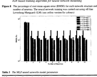
every network structure and hidden neuron case. Subsequently, the stored error calculation was then retrieved at the end of the validation cycle for RMSE computation.

The results of k-fold cross validation for the off-line NN model is given in Figure 8. For each neuron size, different network structures were tested and compared with each other. From the plot, network sti'ucture with 3 past outputs and

I

past input (regression vector or input nodes with dimension size of 8) gives the lowest RMSE value for neurons size,

fr,

:

4. This network structure was then used as the basic architecture for comparing the generalisation performance of the recursive Gauss-Newton method with the

offline

NN model. Note that the neuron size D,

:

8 gives a comparable low RMSE values. However,

(18)

[image:18.593.100.429.99.358.2]

rGN based

taining

algorithm

_for

neural netvvork modelling

Figure

8

The percentage of root mean square elror (RMSE) for each network structure and number of neurons. The neural network training was carried out using offJine Levenberg-Marquardt (LM) (see online version for colours)

Thble

3

The MLP neural networks model parameters MLP nenvork specifications _forattitude dynamics Number ofpast outputs

Number of past inputs

Number of neurons in hidden layer Activation function at hidden layer Activation function at output layer Number of regressors

Total number of weights Weight decay

73

3

I

^ Tanh Linear

a

46 0.0001

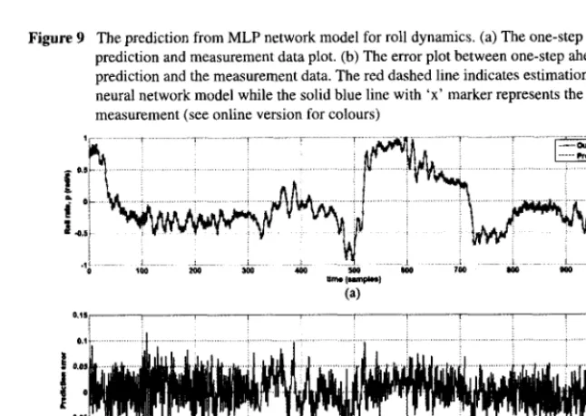
An example ofthe one-step ahead prediction ofthe angular rate responses that are estimated from the

offline

neural network system identification is shown in Figures 9 and 10. The network is trained using the nearly optimal structure from Table 3. These predicted responses

from neural network identification

(NNID)

are overlaid

with

the measured helicopter responses. The results indicate that one-step ahead NNID predictions overlap the test data almost perfectly as indicated by the magnitude order

of

the prediction error plot. This usually happens when the sampling frequency of the data collected is high compared with the frequency ofthe dynamic system as suggested in Norgaard (2000).

This work also utilised the ,k-fold cross validation method to identify the efficiency

of

the selected neural network

raining

methods

in

estimating the attitude dynamics

of

(19)

74

this plot, we consider a network structure of 3 past output and

I

past input as a network structure for both training algorithms. The recursive training algorithm (rGN) exhibits a

slightly higher generalisation error in cross validation compared with the off-line method. This indicates that training performed over a large data set would give better generalisation performance over the recursive method.

Even though the generalisation error of rGN is slightly higher than the

offline

LM, the rGN is more adaptive to the changes in dynamic properties. As a comparative study of the adaptability between the off-line

LM

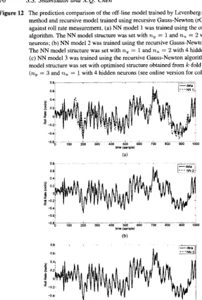
and rGN methods, the roll rate measurement from a new data set is considered. Figure 12 shows the prediction from a pre-trained model using off-line LM and rGN method. The corresponding error statistics for these prediction models is given in Thble 4. In Figure 12(a) and (b), the offJine model (NN

l)

is pre{ained using 1 past output and 2 past inputs with 4 hidden neurons (training with746 samples) while the recursive model (NN 2) is also trained with the same model structure. The training of

rGN is carried out using the sliding window method where older data is discarded from the window to allow present data to enter. Thus, it can be seen that the off-line model follows the output measurement accurately at the beginning of the data length and its prediction begins to deteriorate for the remaining data. Whereas, the prediction from the model trained using rGN algorithm adapts well to the dynamic changes that occur during flight even though

it

was not trained using the optimal structure. In Figure 12(c), the prediction model (NN 3) using the optimal model structure

(n,

:

3, n.u

:

I

with 4 hidden neurons) gives the best RMSE accuracy with t9.454% and 11.611% for roll rate and pitch rate respectively. Note thar the RMSE values for recursive training (NN3) is slightly higher than results obtained

[image:19.592.91.415.398.628.2]

in Figure I

I

since the recursive training is done with a single pass to the data compared with the results obtained in reoeated recursive trainins.

Figure

9

The prediction from MLP network model for roll dynamics. (a) The one-step ahead

prediction and measurement data plot. (b) The error plot between one-step ahead

prediction and the measurement data. The red dashed line indicates estimation from the neural network model while the solid blue line with 'x' marker represents the output measurement (see online version for colours)

hlm9L.) (a)

(b) I

t

I_t

(20)

[image:20.592.107.422.106.357.2] [image:20.592.95.428.120.567.2]

rGN based training aQortthmfor neural netvvork

modelling

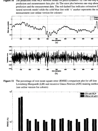
75 Figure

10

The prediction from MLP network model for pitch dynamics. (a) The one-step ahead

prediction and measurement data plot. (b) The error plot between one-step ahead

prediction and the measurement data. The red dashed line indicates estimation from the neural network model while the solid blue line with 'x' marker represents the output measurement (see online version for colours)

Figure

11

The percentage of root mean square error (RMSE) comparison plot for offJine Levenberg-Marquardt (LM) and recursive Gauss-Newton (rGN) training methods (see online version for colours)

I

i

a

s

hlr$b) (b)

IIrGN

with

MLP

i]

llofiine

LM with MLP _I

'l

I

ltilltilililililll

2345678910

(21)

[image:21.594.109.396.104.530.2]

76 S.S. Shamsudin and X.Q. Chen

Figure

12

The prediction comparison of the off-line model trained by Levenberg-Marquardt (LM) method and recursive modei trained using recursive Gauss-Newton (rGN) method against roll rate measurement. (a) NN model I was trained using the off-line LM algorithm. The NN model structure was set with ny

:

1 and nu

:

2 wrth 4 hidden neurons; (b) NN model 2 was trained using the recursive Gauss-Newton algorithm. The NN model structure was set with as

:

I

and nu

:

2 \rtith 4 hidden neurons and (c) NN model 3 was trained using the recursive Gauss-Newton algorithm. The NN model structure was set with optimised structure obtained from ft-fold cross validation

(n,

:

3 andrtu

:

1 with 4 hidden neurons (see online version for colours)

2@ 300

16o s6o

6b

zh tffi (smpl6)

(a)

t-*-t

l--- NN2il

e

E

t 42i

-0.1f

-0.61

"o r00 2m 3m 100 5@ 6@ 76 8m m 1@0 tm (smpl6)

(b)

tfr (smple) (c)

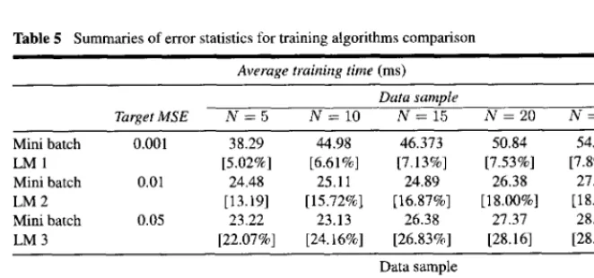
In on-line system identification for adaptive control application, the training time for NN model needs to be less than the sampling time of the control loop. This is essential since the control decisions need to be updated at the specific timing requirement (less than 22 ms). There are two type of recursive algorithm method exists to approximate the non-linear dynamics in real-time:

mini-batch methods (Samal, 2009; Puttige, 2009)

recursive prediction methods as presented in previous section.

{

E fi

-0.8

0.81

o4i

0.2

a

(22)

_for

neural network

modelling

77

For mini-batch wise methods, the off-line training such as

LM

algorithm was used to train the NN in real-time by choosing smaller data length to achieve faster convergence time. Typically, a fixed amount

of

input-output data is collected and stored

in

a queue. Table 5 shows the average training time for mini-batch

LM

and rGN training algorithms for attitude dynamics identification using the optimal NN model structure

(r4

:

3,rlu

: I

with 4 hidden neurons). The minimum criterion enor (MSE) was selected at 0.001, 0.01 and 0.05 as stopping criteria for mini-batch

LM

training. The training time comparison test was conducted using a 400 MHz National Instrument's real-time embedded controller. Result from the comparison test shows that faster training convergence is achieved with smaller batch sizes. However, mini-batch method

still

requires a

lot

more computation resources and would not finish within targeted sampling period (22 ms). Attempts to reduce the training time

of

the NN training through manipulation

of

target MSE values could improve the algorithm training performance, but at the expense

of

poor training error. A recursive training algorithm such as rGN usually demonstrates faster prediction updates and offers rapid computation of weight adaptation with average training time of 3.88 ms. The average training time forrGN algorithm is well below the control loop sampling period (22 ms) and this indicates that such recursive training algorithms are well suited for real-time applications.

Table

4

Summaries of error statistics fbr training algorithms comparison Error statistic's

Training System responses RMSE RMSE (Vo\ R"

NNI

p q 0.08891 0.03495 42.376 16.65'7 0.8506 0.964'7 NN2 D q 0.04907 0.03665 23.366 t7.454 0.9451 0.969r NN3 D q 0.09289 0.04244 19.454 I 1.61 1

0.9620 0.9863

Table

5

Summaries of error statistics for training algorithms comparison Average training time (ms)

Target MSE Mini batch

LMI

Mini batch L]|d2 Mini batch

LM3

0.001

0.01

0.05

[image:22.594.100.431.332.436.2] [image:22.594.100.431.468.623.2]

38.29

44.98

[5.02Eo]

16.617o)

24.48

25.11

t13.i9l

l15.72qol

23.22

23.13 122.0'7%ol [24.r6%al

46.373 50.84

54.78

[1.I3Eol

11

.53%ol

l7.89Voj

24.89

26.38

27.53

116.8'lEol

[18.007o]

U8.471

26.38

27.37

28.86

l26.83Sal

t28.161

t28.481 Data sample

N=1

rGN 3.88

(23)

78 8

Conclusion

The methods and results presented in this paper indicate the suitability and effectiveness

of

offline

and recursive based neural network modelling

for

representing coupled

UAS helicopter dynamics

with

acceptable accuracy. Results indicate that although the generalisation error of rGN is slightly higher than off-line

LM,

the rGN is more adaptive

to

the changes

in

dynamic properties. The rGN method

is

also capable to produce a satisfactory prediction quality even-though the model structure was incorrectly selected. The generalisation and adaptability performance can be further improved by properly selecting the optimised network structure with the aid of k-fold cross validation method. It can also be concluded that the recursive method presented here is suitable to model the UAS helicopter

in real-time within the computational resource constraints. These models can be further used for the design of adaptive flight controllers for autonomous flight.

Acknowledgement

S.S. Shamsudin acknowledges financial support

from Ministry

of

Higher Education, Malaysia under

IPTA

Academic Training Scheme. The authors would

like to

thank technicians in Mechanical Engineering Department, University of Canterbury, in particular, Julian Mulphy and David Read for their invaluable assistance and support to our research project. The authors also

like

to thank the reviewers

for

their suggestions which have improved the quality of the presentation.

References

Agarwal, M. (1997) 'A systematic classification of neural-network-based control', Control Systerns,

IEEE,YoI. 17, No. 2, pp.75-93.

Balakrishnan, S.N. and Weil, R.D. (1996) 'Neurocontrol: a literature suruey', Mathematical and ComputerModelling,Yol.23,Nos. l-2,pp.l0l-117,doi:10.1016/0895-7177(95)00221-9. Bierman, G.J. (1977) Factorization Methods

_for

Discrete Sequential Estimation, Volume 128,

Academic Press, New York.

Billings, S.A., Jamaluddin, H.B. and Chen, S. (1991) 'A comparison of the backpropagation and recursive prediction error algorithms for training neural networks', Mechanical Systems and Signal Processing, Vol 5, No. 3, pp.233-255.

Billings, S.A., Jamaluddin, H.B. and Chen, S. (1992) 'Properties of neural networks with applications to modelling non-linear dynamical systems'. International. Journal of Control, Vol. 55, No. 1,

pp.193-224.

Budiyono, A., Joon, YK. and Daniel, F.D. (2009) 'Integrated identification modeling of rotorcraft-based unmanned aerial vehicle', lTth Mediterranean Conference on Control and Automation, 24-26 June, IEEE, Thessaloniki, Greece, pp.898-903.

Calise, A.J. and Rysdyk, R.T. ( 1998) 'Nonlinearadaptive flightcontrol using neural networks' , Control

Systems, IEEE,YoI. 1 8, No. 6, December, pp. 14-25, ISSN 1066-033X, doi: 10.1 109/37.736008.

(24)

_for

neural network

modelling

79 Jiang, 2., Han, J.D., Wang, YC. and Song, Q. (2006) 'Enhanced LQR control for unmanned helicopter

in

hover', Ist International Symposium on Systems and Control in Aerospace

and Astronautics, 2006. ISSCM 2006. Ianuary. Harbin, China, pp.1438-l'143' doi:

10. 1 10945SCAA.2006. l 627s08.

Kendoul, F. (2012)'survey of advances in guidance, navigation, and control of unmanned rotorcraft systems', Joumal of Field Robotics, Vol. 29, No. 2, pp.315-378, ISSN 1556-4967.

Kohavi, R. (1995) 'A study of cross-validation and bootstrap for accuracy estimation and model selection',I/re 1995 InternatiortalJointConferenceonArtificiallntelligence,MorganKaufmann Publishers Inc., San Francisco, CA, USA, pp. I 137-1 145.

Ljung, L. (1999) System Identifcation: Theory _forthe lJser,2nd ed., Prentice Hall information and system sciences Series, Prentice Hall PTR, Upper Saddle River, NJ.

Ljung, L. and Soderstrom, T. (1983) Theory and Practice of Recursi't,e ldentifcation, The MIT Press series in signal processing, optimization, and control, MIT Press, Cambridge, Mass.

Mettler, B. (2003) Identification Modeling and Characteristics of Miniature Rotorcraft,

ls|

ed.,

Kluwer Academic Publishers, Boston.

Ngia, L.S.H. and Sjoberg, J. (2000) 'Efficient training of neural nets for nonlinear adaptive filtering using a recursive levenberg-marquardt algorithm', IEEE Transactions on Signal Processing, Vol. 48, No. 1 _,pp.19l5-1927 .

Norgaard,

M.

(2000) Neural. Nerworks

_for

Modelling and Control

of

funamit' Systems: A Practitioner's Harulbook,2nded.,Advanced textbooks in control and signal processing, Springer, Berlin, New York.

Putro, I.E., Budiyono, A., Yoon, K.J. and Kim, D.H. (2009) 'Modeling of unmanned small scale

rotorcraft based on neural network identification', 2008 IEEE International Conference on Robotics and Biomimetics, Bangkok, Thailand, pp. 1938-1943.

Puttige, V.R. and Anavatti, S.G. (2006) 'Real-time neural network based online identilication technique for a UAV platform', Intenwtional Conference on Computational futellig,ence

_for

Modelling, Control and Automation, 2006 and International Confurence on InteLligent Agents, Web Technologies and Intemet Commerce, Sydney, NSW p.92-92.

Puttige, V.R. (2009) Neural Nenvork based Adaptive Conftol for Autonomous Flight of Fixed Wing (Jnnanned AerietlVehicles,PhDThesis, School ofAerospace, Civil andMechanicalEngineering, Australian Defence Force Academy, University of New South Wales, August 2009, URL: http://handle.unsw.edu.au/l 959. 41 437 36.

Salgado, M.E., Goodwin, G.C. and Middleton, R.H. (1988) 'Modified least squares algorithm incorporating exponential resetting and forgetting', Intemational Journal of Control, Yol. 47, No.2, pp.477491, URL: http://wwwtandfonline.com/doi/abs/10.1080/00207178808906026. Samal, M.K., Anavatri, S. and Garratt, M. (2009) 'Real-time neural network based identification of a

rotary-wing UAV dynamics forautonomous flight' , IEEE International Conference on Industrial Technology,2009. ICIT 2009, Gippsland, VIC, pp.1-6.

Samal, M. (2009) Neural Network based Identification and Control of an Unmanned Helicopter,PhD Thesis, School of Engineering and Information Technology, University of New South Wales, Sydney. NSW Australia.

Samal, M.K., Anavatti, S. and Ganatt, M. (2008) 'Neural network based system identification for autonomousflightofaneaglehelicopter', lTthWorMCongressThelntemationaLFederationof Autotnatic Co n trol, Yol. 17, pp.7 421-7 426.

Samarasinghe, S .(2007) Neural NetworksforApplied Sciences and Engineering: From Fundamentals

to Complex Pattern Recognition,

lst

ed.. Auerbach Publications, Boca Raton, FL, ISBN

08493337 5X, 97 808493 33750.

(25)

80

Shim, D.H. (2000) Hierarchical Flight Control System Synthesis for Rotorcraft based Unmanned Aerial Vehicles, PhD Thesis, University of California, Berkeley.

Sjoberg, J., Zhang, Q.H., Ljung, L., Benveniste, A., Delyon, B., Glorennec, P-Y., Hjalmarsson, H. and Juditsky, A. (1995) 'Nonlinear black-box modeling in system identification: a unified overview',

Automatica Vol. 31, No. 12, pp.169l-1724.

Suresh, S., Kumar, M.V., Omkar, S.N., Mani, V. and Sampath, P (2002) 'Neural networks based

identification of helicopter dynamics using flight data', 9th International Conference on Neural Information Processing ICONIP (2002),Vol. I, pp.l0-14.

Tischler, M.B. and Remple, R.K. (2006) A ircraft and Rotorcraft Systenr ldefiirtcafion : Engineering Metlnds with Flight-T?st Examples, AIAA education series. American Institute of Aeronautics and Astronautics. Reston, VA, 2006.

Wilamowski, B.M. (2009) 'Neural network architectures and learaing algorithms', Industrial Electronics Magazine, IEEE, Vol. 3, No. x, pp.56-63.

Youmin, Z. and R. Li. X. (1999) A fast U-D factorization-based leaming algorithm with applications to nonlinear system modeling and identilication' , IEEE Transactions on Neural Neflt,orks,Yol.10,

No.4, pp.930-938.