Active Noise Cancellation in Audio Signal Processing

© 2016, IRJET | Impact Factor value: 4.45 | ISO 9001:2008 Certified Journal | Page 21

Active Noise Cancellation in Audio Signal Processing

Atar Mon

_{, Thiri Thandar}

_Aung

_{, Chit Htay Lwin}

1

_{Yangon Technological Universtiy, Yangon, Myanmar}

2

_{Yangon Technological Universtiy, Yangon, Myanmar}

_{D.S.A, Pyin Oo Lwin, Myanmar}

---***---

Abstract -

Key Words:active noise cancellation, audio signal processing, adaptive filters, LMS, NLMS, RLS

1. INTRODUCTION

Noise can be defined as an unwanted signal that interferes with the communication or measurement of another signal. A noise itself is an information-bearing signal that conveys information regarding the sources of the noise and the environment in which it propagates. The types and sources of noise and distortions are many and include: (i) electronic noise such as thermal noise and shot noise, (ii) acoustic noise

emanating from moving, vibrating or colliding sources such as revolving machines, moving vehicles, keyboard clicks, wind and rain, (iii) electromagnetic noise that can interfere with the transmission and reception of voice, image and data over the radio-frequency spectrum, (iv) electrostatic noise

generated by the presence of a voltage, (v) communication channel distortion and fading and (vi) quantization noise and lost data packets due to network congestion [1].

The rest of the paper is organized as follows: Section 2 reviews some adaptive filtering methods and analyzed how to cancel the background noise of audio signal processing. The explanation of adaptive algorithms is described in section 3. The test and result of simulation for active noise cancellation and comparison of adaptive algorithms are presented in section 4. Section 5 concludes the paper.

2. BACKGROUND

Noise and degradation are the main factors that limit the capacity of audio signal processing, communication and the accuracy of results in signal measurement systems. Therefore the modeling and removal of the effects of noise and distortions have been at the core of the theory and practice of signal processing and communications. Noise reduction and degradation removal are important problems in applications such as audio signal processing, cellular mobile communication, speech recognition, image processing, medical signal processing, radar, sonar, and in any application where the desired signals cannot be isolated from noise and distortion or observed in isolation.

2.1 Noise control systems

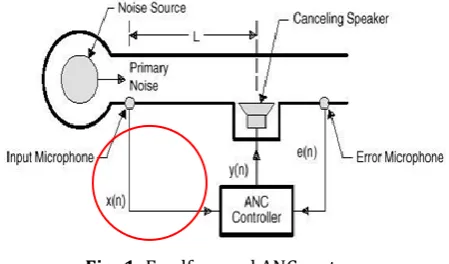
There are two basic types of noise control systems used to analyze the noise and generate the correct inverse signal of the offending sound. The first type of active sound control system is the most widely used presently in existence.

The adaptive feedforward system in Fig.1 is named because a reference sensor samples the noise and feeds it forward to the control system where the noise is filtered by an electronic controller. Then the signal is analyzed and the

© 2016, IRJET | Impact Factor value: 4.45 | ISO 9001:2008 Certified Journal | Page 22

output source. Further down the sound’s path of travel an error sensor again samples the residual sound pressure and provides a signal to the control algorithm to measure controller effectiveness and appropriately adjust the output to obtain the minimization of error, or, physically, the minimization of any residual sound pressure.

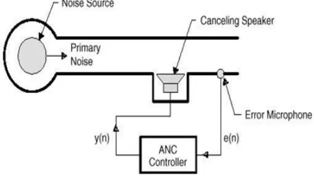
The second type of control system is the active feedback control system as shown in Fig.2. The difference between the two systems is how the control signal is derived. Where the feedforward system samples the sound first, the sound has already passed the electronic controller when it’s sampled by the error microphone in a feedback system and then the signal is sent back to the electronic controller to be analyzed.

2.2 Background Noise

In acoustics and specifically in acoustical engineering, background noise or ambient noise is any sound other than the sound being monitored (primary sound). Background noise is a form of noise pollution or interference. Background noise is an important concept in setting noise regulations. Examples of background noises are environmental noises such as waves, traffic noise, alarms, people talking, bioacoustics noise from animals or birds and mechanical noise from devices such as refrigerators or air conditioning, power supplies or motors. The prevention or reduction of background noise is important in the field of active noise control. It is also an important consideration with the use of ultrasound (e.g. for medical diagnosis or imaging), sonar and sound reproduction.

2.3 Adaptive filtering

Adaptive linear filters are linear dynamical system with variable or adaptive structure and parameters. They have the property to modify the values of their parameters, i.e. their transfer function, during the processing of the input signal, in order to generate signal at the output without undesired components, degradation, noise and interference signals.

2.3.1 Adaptive Noise Cancellation

In speech communication from a noisy acoustic environment such as a moving car or train, or over a noisy telephone channel, the speech signal is observed in an additive random noise. In signal measurement systems the information-bearing signal is often contaminated by noise from its surrounding environment. The noisy observation

y(m) can be modeled as

y(m)=x(m)+n(m)

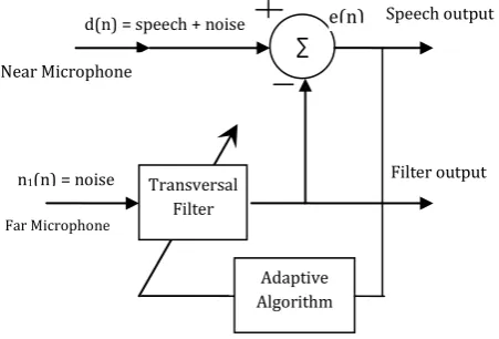
where x(m) and n(m) are the signal and the noise, and m is the discrete-time index. In some situations, for example when using a mobile telephone in a moving car, or when using a radio communication device in an aircraft cockpit, it may be possible to measure and estimate the instantaneous amplitude of the ambient noise using a directional microphone. The signal x(m) may then be recovered by subtraction of an estimate of the noise from the noisy signal. Fig. 3 shows a two-input adaptive noise cancellation system for enhancement of noisy speech. In this system a directional microphone takes as input the noisy signal x(m) +

n(m), and a second directional microphone, positioned some distance away, measures the noise α n(m+τ).

The attenuation factor α and the time delay τ provide a rather over-simplified model of the effects of propagation of the noise to different positions in the space where the microphones are placed. The noise from the second microphone is processed by an adaptive digital filter to make it equal to the noise contaminating the speech signal, and then subtracted from the noisy signal to cancel out the noise.

2.3.2 Active Noise Cancelling

The active noise cancelling, also called adaptive noise cancelling or active noise canceller belongs to the interference cancelling class.

Fig -3: A two-microphone adaptive noise canceller

© 2016, IRJET | Impact Factor value: 4.45 | ISO 9001:2008 Certified Journal | Page 23

is to minimize the noise interference or, in an optimum situation, cancel that perturbation [2].

The approach adopted in the ANC algorithm, is to try to imitate the original signal x(n). A scheme of the ANC can be viewed in Fig.4. In the ANC, as explained before, the aim is to minimize the noise interference that corrupts the original input signal. In the figure above, the desired signal d(n) is composed by an unknown signal, that s(n) is called corrupted for an additional noise n2(n), generated for the

interference. The adaptive filter is then installed in a place that the only input is the interference signal n1(n).

The signals n1(n) and n2(n) are correlated. The output of the filter y(n) is compared with the desired signal d(n), generating an error e(n). That error, which is the system output, is used to adjust the variable weights of the adaptive filter in order to minimize the noise interference. In an optimal situation, the output of the system e(n) is composed by the signal s(n), free of the noise interference n2(n). In the ANC, as explained before, the aim is to minimize the noise interference that corrupts the original input signal.

2.3.3 Adaptive Filters

As their own name suggests, adaptive filters are filters with the ability of adaptation to an unknown environment. This family of filters has been widely applied because of its versatility (capable of operating in an unknown system) and low cost (hardware cost of implementation, compared with the non-adaptive filters, acting in the same system).

The ability of operating in an unknown environment added to the capability of tracking time variations of input statistics makes the adaptive filter a powerful device for signal-processing and control applications. Indeed, adaptive filters can be used in numerous applications and they have been successfully utilized over the years [3].

As it was before mentioned, the applications of adaptive filters are numerous. For that reason, applications are

separated in four basic classes: identification, inverse modeling, prediction and interference cancelling.

All the applications above mentioned, have a common characteristic: an input signal is received for the adaptive filter and compared with a desired response, generating an error. That error is then used to modify the adjustable coefficients of the filter, generally called weight, in order to minimize the error and, in some optimal sense, to make that error being optimized, in some cases tending to zero, and in another tending to a desired signal.

An adaptive filter is defined by four aspects:  The signals being processed by the filter

 The structure that defines how the output signal of the filter is computed from its input signal

 The parameters within this structure that can be iteratively changed to alter the filter’s input-output relationship

 The adaptive algorithm that describes how the parameters are adjusted from one time instant to the next

3. ADAPTIVE ALGORITHMS

Adaptive algorithms are useful for adaptation of digital filters. The conventional adaptive algorithms (RLS, LMS, NLMS) are analyzed in this section.

3.1 Recursive Least Square Algorithm (RLS)

The recursive least square (RLS) algorithm [4, 5] was proposed in order to provide superior performance compared to those of the LMS algorithm and its variants [6, 7], with few parameters to be predefined, especially in highly correlated environments. In the RLS algorithm, an estimate of the autocorrelation matrix is used to decorrelate the current input data.

Even though the RLS algorithm has very good performance in such environments, it actually suffers from its high computational complexity. Also, in RLS algorithm, the forgetting factor  has to be chosen carefully such that its value should be very close to one in order to ensure stability and convergence of the RLS algorithm.

where, x(n) is the input vector of time delayed input values,

w(n) represents the coefficients of the adaptive FIR filter tap weight vector at time n and k(n) is a function of forgetting factor correlation matrix (n).

d(n) = speech + noise

∑

Transversal Filter

Adaptive Algorithm Near Microphone

e(n)

n1(n) = noise

Far Microphone

Speech output

Filter output

© 2016, IRJET | Impact Factor value: 4.45 | ISO 9001:2008 Certified Journal | Page 24

algorithm because small values of  may be required for signal tracking if the environment is non-stationary [8].

3.2 Least-Mean-Square Algorithm (LMS)

The LMS algorithm [9], is a stochastic gradient-based algorithms as it utilizes the gradient vector of the filter tap weights to converge on the optimal wiener solution. With each iteration of the LMS algorithm, the filter tap weights of the adaptive filter are updated according to the following formula:

w ( n 1 ) w ( n ) 2µe( n ) x ( n )

where, x(n) is the input vector of time delayed input values,

w(n) represents the coefficients of the adaptive FIR filter tap weight vector at time n and μ is known as the step size.

Selection of a suitable value for μ is imperative to the performance of the LMS algorithm, if the value μ is too small, the time adaptive filter takes to converge on the optimal solution will be too long; if μ is too large the adaptive filter becomes unstable and its output diverges.

3.3 Normalized Least-Mean-Square Algorithm (NLMS)

In the standard LMS algorithm, when the convergence factor μ is large, the algorithm experiences a gradient noise amplification problem. This difficulty is solved by NLMS (Normalized Least Mean Square) algorithm. The correction applied to the weight vector w(n) at iteration n+1 is “normalized” with respect to the squared Euclidian norm of the input vector x(n) at iteration n.

The NLMS algorithm can be viewed as a time-varying step-size algorithm, calculating the convergence factor μ as follows [4].

where α is the NLMS adaption constant, which optimize the convergence rate of the algorithm and should satisfy the condition 0<α<2, and c is the constant term for normalization, which is always less than 1.

3.4 The Modified Adaptive Algorithm

Normalized Least Mean Square algorithm is modified and implemented using sign function in adaptive noise cancellation.

The sign of real number, also called sign or signum is (-1)

for a negative number (i.e one with a minus sign “ – ”, 0 for

the number zero, or +1 for a positive number (i.e, one with a plus sign “ + ”).

In other words for real x

for real x0, it can be written as;

4. SIMULATION AND PERFORMANCE ANALYSIS

This section describes how the proposed system is developed and followed by a detailed explanation of the architecture of the system.

4.1 Active Noise Cancellation of Audio Signal

Processing

The active noise cancelling (ANC), also called adaptive noise cancelling or active noise canceller belongs to the interference cancelling class. The aim of this algorithm is to minimize the noise interference or, in an optimum situation, cancel that perturbation.

Begin NLMS

Initialize of variables

Read input noise x(n),

noisy signal d(n)

variables

V Calculate NLMS

Begin Filtering, calculate error e(n ) = d(n)-y(n)

Update Weight vector w

n = n+1

n = 0 Time index n =

Length N No

Yes

© 2016, IRJET | Impact Factor value: 4.45 | ISO 9001:2008 Certified Journal | Page 25

imitate the original signal x(n). In this study, the final objective is to use an ANC algorithm to cancel background noise interference, but this algorithm can be employed to deal with any other type of corrupted signal. A scheme of the ANC can be viewed in Fig 5.

4.2 Performance Measures in Adaptive Systems

Some important measures will be discussed in the following:

4.2.1 Convergence Rate

The Convergence rate determines the rate at which the filter converges to its resultant state. Usually a faster convergence rate is a desired characteristic of an adaptive system. Convergence rate is not independent of all the other performance characteristics. There is usually a tradeoff, with convergence rate and other performance criteria [2].

4.2.2 Mean Square Error (MSE)

The MSE is a metric indicating how much a system can adapt to a given solution. A small MSE is an indication that the adaptive system has accurately modeled, predicted, adapted and/or converged to a solution for the system. There are a number of factors which will help to determine the MSE including, but not limited to; quantization noise, order of the adaptive system, measurement noise, and error of the gradient due to the finite step size [4].

Error = Desired signal – Enhanced signal e(n) = d(n) – y(n), then MSE is

4.2.3 Computational Complexity

Computational complexity is particularly important in real time adaptive filter applications. When a real time system is being implemented, there are hardware limitations that may affect the performance of the system. A highly complex algorithm will require much greater hardware resources than a simplistic algorithm [8].

4.2.4 Log Spectral Distance

The log spectral distance (LSD), also referred to as log-spectral distortion, is a distance measure between two spectra. It calculates the average log-spectral distance between clean and noisy signals. The lower LSD, the higher the amount of noise cancellation.

The log spectra are much closer to the parameters used in a discriminator than power spectra. This spectral estimation

performed better than spectral subtraction in noise immunity experiment.The log spectral distance between spectra P(w) and is defined as

where P(w) is average power of noisy signal and is average power of input signal.

4.2.5 Noise Reduction Ratio(NRR)

A representative part of the Noise Reduction Ratio (NRR) is defined as the ratio of average power of reference noise signal to error signal. It measures that how much noise is reduced from background. Note that NRR is calculated after the filter adaptation is finished (stationary condition) [3].

,

4.3 Simulation

RLS, LMS, NLMS and modified NLMS are implemented for Active Noise Caioncellation using MATLAB simulation. It is also given the result of each algorithm applied for performance of experiments and a comparison between those results. The background noise is in the nature of Gaussian noise. So, this noise is added to 300Hz of audio signal. All simulated results are observed by 10000 iterations. Filter length 10 is used to obtain better performance.

(a) (b)

(c)

Fig -6: Comparison of MSE for (a) LMS, (b) NLMS and (c) modified NLMS ( = 0.005)

M

ea

n

S

q

u

are

Err

o

r

(d

B)

© 2016, IRJET | Impact Factor value: 4.45 | ISO 9001:2008 Certified Journal | Page 26

convergent rate of modified NLMS is faster than NLMS algorithm in stability condition.

4.3.1 Analysis of RLS, LMS, and NLMS algorithms

The analysis of the four algorithms will be performed according to the factors presented in the section 4.2. They are convergence rate, MSE, log spectral Distance and the NRR.

Fig.7 and Fig.8 show modified algorithm is better performance than LMS and NLMS algorithm. Therefore, noise can be reduced more than NLMS algorithm in Fig.9.

5. CONCLUSION

The simulation results are being performed at (µ=0.005) for a modified algorithms, NLMS, LMS algorithm and RLS algorithm. The performance of these four algorithms was investigated for broadband (10Hz-4GHz) background noise as the nature of Gaussian white noise distribution. The convergence performance of the regular LMS algorithm was compared to the normalized LMS variants.

The convergent rate of LMS is the fastest but it is not good resolution. The normalized version adapts in far fewer iterations to a result almost as good as the nonnormalized version. Adaptive filters and algorithm are described in overview emphasizing the applications.

The modified NLMS algorithm is three times faster than NLMS algorithm. Amount of Nose is reduced 5dB more than LMS. But it is less than RLS algorithm. Lower amount of noise cancellation was obtained than LMS and NLMS according to log spectral distance. MSE is also less than NLMS. But, LMS algorithms is less resolution than modified NLMS at (µ=0.005). Therefore, modified NLMS is recommended better performance than LMS and NLMS algorithm.

The advantages of Active Noise Cancellation (ANC) system are efficiently attenuating low frequency noise where passive methods are either ineffective. Basic algorithms that have already proven themselves are to be useful in practice. Despite the many contributions in the field, research efforts in adaptive filters continue at a strong pace.

It is likely that new applications for adaptive filters will be developed in the future. This implies that the proposed algorithm can significantly reduce the cost of implementation of adaptive systems.

The proposed continuation of this work is to build a prototype of the ANC using the modified NLMS algorithm. The program would be converted to C programming language or any other programming language compatible with the controller.

REFERENCES

[1] Saeed V. Vaseghi, ‘‘Advanced Digital Signal Processing and Noise Reduction’’, Fourth Edition John Wiley& Sons, Ltd., 2013.

[2] Lakshmikanth.S, “An Novel Approach for Noise Cancellation in Industrial Environment”, Ph.D. Thesis, Department of Electronics and Electrical Engineering, Jain University, Bangaluru, 2015.

[3] Per Rubak, Henrik D. Green and Lars G. Johansen, “Adaptive Noise Cancellation in Headsets”, Aalborg University, Institute for Electronic Systems, 2013. [4] Haykin, Simon, ‘‘Adaptive Filter Theory’’, Prentice Hal,

ISBN 0-13-048434-2, 2002.

[5] Hansen, C.H., ‘‘Understanding Active Noise Cancellation’’, New York: Spon Press, 2001.

Fig -7: Comparison of Log spectral distance for Four Algorithms

Log

spe

ctr

al

dista

nc

e

(dB)

N

oise

R

educ

tion

R

atio

(dB)

Fig -8: Comparison of Noise

Reduction Ratio for Four Algorithms

Me

an

Sq

ua

re

E

rr

or

(

-dB)

© 2016, IRJET | Impact Factor value: 4.45 | ISO 9001:2008 Certified Journal | Page 27

and Applications”, Second Edition, University of Utah, USA, 2013.

[7] Bartholomae, R.C., & Stein, R.R. ‘‘Active noise cancellation – performance in a hearing protector under ideal and degraded conditions’’, Austin: University of Texas, 1990.

[8] Jyoti Dhiman, ‘‘Comparison between Adaptive filter Algorithms’’, International Journal of Science, Engineering and Technology Research (IJSETR) Volume 2, Issue 5, May 2013.