An Online Malicious Spam Email Detection System Using Resource Allocating Network with Locality Sensitive Hashing

http://dx.doi.org/10.4236/jilsa.2015.72005

An Online Malicious Spam Email Detection

System Using Resource Allocating Network

with Locality Sensitive Hashing

Siti-Hajar-Aminah Ali

1

, Seiichi Ozawa

1

, Junji Nakazato

2

, Tao Ban

2

, Jumpei Shimamura

3 1_{Graduate School of Engineering, Kobe University, Kobe, Japan}

2_{National Institute of Information and Communications Technology (NICT),Tokyo, Japan} 3_{Clwit Inc.,Tokyo, Japan}

Email: [email protected], [email protected], [email protected], [email protected], [email protected]

Received 25 February 2015; accepted 20 April 2015; published 22 April 2015

Copyright © 2015 by authors and Scientific Research Publishing Inc.

This work is licensed under the Creative Commons Attribution International License (CC BY). http://creativecommons.org/licenses/by/4.0/

Abstract

Keywords

Malicious Spam Email Detection System, Incremental Learning, Resource Allocating Network, Locality Sensitive Hashing

1. Introduction

Emails have become one of the most frequently used methods for cyber attacks. The most worrying email-based attack is Targeted Malicious Email (TME) [1] [2]. In TME, attackers send malicious emails to certain people targeted in an organization, such as executives of large companies, high-ranking government personnel, military officials and even famous researchers, in order for the attackers to obtain valuable confidential information and latest research of the targeted people. In TME, an email often has an attachment with malicious codes that can be installed automatically upon opening without the victims realizing it. In some cases, the victims’ computer will become the back door for the attackers who in turn have the authority to enter the network of the targeted persons and thus steal confidential information.

Another typical email-based cyber attack is the malicious spam email attack, which aims to spread numerous emails with Uniform Resource Locator (URL) links leading to malicious websites. Previously, malicious codes were sent through the attachment of such spam emails. However, many successful filters have been developed to detect malicious attachments. Thus, attackers are now turning to malicious spam campaigns that attack using the links attached in the emails. According to the Symantec annual report in 2014 [3], about 87 percent of scanned spam messages contained at least one URL hyperlink. Moreover, recent findings by Symantec [4] show a sharp rise of emails containing malicious links, from 7% in October 2014 to 41% in the following months. Apart from that, currently, attackers also use more relevant email contents [1] that are specific to their victims’ line of work, besides addressing the name of the recipient in the email body to convince the victim that the email received is a normal email. For instance, a fake email notification regarding a conference or journal targeted towards a recipient with academic status, notifications regarding false documents such as telecommunication service bills, fax and voicemail in which the victims are given a link to get more information [4]. This technique is called Social Engineering [5], which Hadnagy [6] defines as “The Art of Human Hacking”. It becomes difficult for normal users to distinguish not only between non-malicious and malicious spam emails but also spam email from normal emails.

The objective of this paper is to detect the malicious spam emails so that general users can be protected from being re-directed to malicious websites. For this purpose, we propose an autonomous online system for detecting malicious spam emails. In general, it is not easy to collect spam emails from individual persons because it is not usually permitted to access personal email spools. Therefore in the proposed system, we collect double-bounce spam emails that are delivered to unknown users. From the collected spam emails data, a classifier model is used to learn and classify the malicious spam emails. The updated connection weights of the classifier model are sent to a user’s mailer software to improve the malicious spam email detection ability. Jungsuk [7] points out that the live period of malicious URLs is often very short, usually within a few days; thus, it is expected that introducing incremental learning to malicious spam email detection will be effective. The system can learn from the recent spam emails so that the spam email detection system is always up to date. On the other hand, spammers often use botnets to spread spam emails. For example, a botnet called Rustock which consists of approximately 1 million infected computers that networked together, is capable of sending up to 30 billion spam emails every day [8]. Since the distribution of such spam emails is done in a short time, we assume that the spam emails have the same or similar contents in general [9]. Hence, we adopt the Locality Sensitive Hashing (LSH) [10]-[14] to quickly select important training data to be learned. For this purpose, we adopt Resource Allocating Network with Locality Sensitive Hashing (RAN-LSH) as a classifier model in the proposed detection system. This model has the following two important properties: 1) the learning is carried out incrementally; and 2) only data within an untrained region are selected and learned even when a large amount of data is given.

44

[image:3.595.87.544.417.689.2]

2. Resource Allocating Network with Locally Sensitive Hashing (RAN-LSH)

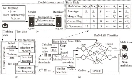
1

Figure 1 demonstrates the overall architecture of the spam email detection system. In this section, we give a brief explanation of the RAN-LSH classifier [15] illustrated in Figure 1(c). RAN-LSH is the extended model of the Resource Allocating Network (RAN) [16], where LSH is adopted to select essential training data and Radial Basis Function (RBF) bases for fast learning. There are three main components in RAN-LSH: hash table, data selection and classifier.

Algorithm 1shows the overall learning procedures of RAN-LSH. During the initial learning phase (Lines 1 - 5), initial training data are used to obtain the most suitable values of the following two important parameters: RBF width

σ

and the number of partitions P. In addition, initial data are also used to obtain an initial hash table and initial structure of the classifier. After that, the incremental learning is carried out whenever training data are given to learn (Lines 7 - 17). In LSH, similar data are allocated in the same hash entry with a high probability. Therefore, the number of hash entries determines the granularity of input space representation, and too large number of hash entries would result in both high computational and memory costs in the data selection. Therefore, it is important to design the hash functions such that a suitable number of hash entries are created.

In RAN-LSH, we adopt Principal Component Analysis (PCA) to generate a proper number of hash functions by controlling the threshold of the accumulation ratio θ_a. Accumulation ratio A U

( )

_l is the ratio of input components in the approximated subspace over those in the whole input space [17]. Giving a proper value of

a

θ based on a tolerant approximation error, a proper number of hash functions is automatically determined by selecting the number of partitions P via the cross-validation.

Let l be the subspace dimensions obtained by PCA. Then, the following linear transformation is considered to define hash values in LSH:

T l

=

V U x (1) where V =

{

v₁,,vl

}

, U=

{

u1,,ul

}

and

x

are the l-dimensional projection vector, the matrix of l

eigenvectors, an I-dimensional input vector, respectively. Each projection vectors v ii

(

=1,,l

)

is then divi-

Figure 1. Network structure of the proposed autonomous malicious spam email detection system.

ded into P partitions with equal size. θ_a controls the number of eigenvectors U_l. To obtain a hash code, data is first projected on all the eigenvectors u_i and the hash code is obtained by combining the encoded values for the projections. When a large θ_a is adopted, the number of eigenvectors tends to become large and this would cause elongation of the length of a hash code.

As shown in Algorithm 1(see Lines 7 - 17), the incremental learning of RAN-LSH is carried out not only for RAN-LSH classifier but also for the hash table. Let us briefly explain the learning procedures in the following subsections.

2.1. Updating Hash Table

Algorithm 2 illustrates the steps to create and update the hash table which is used in RAN-LSH learning algorithm (Lines 4, 8 and 17 in Algorithm 1). Each subregion is allocated to an entry in a hash table, where each entry is composed of five items: hash value h x

( )

_e , prototype x_e, margin flag F_eM, outlier flag F_eO

and the occurrence frequency N_e (Figure 1: top right). The index or a hash value is used as a key to find a matched entry

e

of a similar item which has been registered previously in hash table (see the first condition in Line 6). Hash values h x

( )

=

{

H v

( )

₁ ,,H v

( )

_l

}

are a set of hash functions H v

( )

_i , which are given as follow:

( )

i max min max

{

{ }

i, i , i

}

i ,1

i i

v v v v

H v P

v v

− + −

+ −

 ₋  

_{ } 

= _{ }

 − 

_{ } 

 

(2)

where v_i+ and v_i− are the upper and lower values of projections v_i on the ith eigenvector u_i, respectively. Here, P is the number of partitions which determines the granularity for a projection v_i.

The next item is prototype x_e. A prototype is the mean vector of all data allocated to each entry (Lines 7 and 11) which is calculated as follows:

(

)

( )

1 n

e e i

i e

e

N

N n

=

′ ∗ +

=

+

∑



x x

where x_e′ and x_i are the previous prototype which is registered in the entry

e

and training data that belong to

s

th subset of unique hash values x_i∈X_s, respectively. Meanwhile, N_e is the previous occurrence frequency of the entry

e

and

n

is the number of training data that has a similar hash value. x_e is regarded as the representative point of the subregion.

The third item is the margin flag M e

F and it is calculated as follows (Line 12):

( )

(

)

(

)

0,

1, otherwise

e m

M e

z F =  ∆ ≤θ



x

(4)

where the output margin ∆z is given by subtracting the second largest network output z_k′′

( )

x_e from the

largest network output z_k′

( )

x_e as follows:

( )

{1, , }

( )

{1, , }\

( )

arg max arg max

e k e k e

k K k K k

z z_′ z_′′

′∈ ′′∈ ′

∆ = −

 

x x x (5)

The fourth item is the outlier flag F_eO which is determined as follows (Line 12):

(

)

( )

(

)

(

)

0, 0

0, &

1, otherwise

M e O

e m e o e N

F

F θ z θ N θ

 ₌



=_ ≤ ∆ < <

 

x (6)

The last item is the occurrence frequency N_e of similar data in an entry. Whenever a new training data is

assigned to an entry, the occurrence frequency is increased by one. The details of margin flag F_eM and outlier flag F_eO are discussed in the following Section 2.2 and 3.4, respectively.

2.2. Data Selection and RBF Bases Selection Using LSH

as quickly as possible; otherwise, the next data may be given before the learning is completed. In RAN-LSH, the data selection is conducted by using LSH. First, all N_d training data in a given training set are projected to l

eigenvectors. Then, for each training data, the projection value is encoded into a hash code whose granularity is determined by the number of partitions P, and the obtained hash codes are transformed into a hash value.

If a matched entry with the same hash value is found and the margin flag F_eM is “1”, it means the classifier is well trained (Line 6 in Algorithm 2). Then, the mean vector is calculated and the occurrence frequency N_e

is incremented by

n

. Otherwise (Line 10 in Algorithm 2), the output margin ∆z in Equation (5) is calculated and the margin flag F_eM and outlier flag F_eO are updated by Equations (4) and (6), respectively. Note that the

training data associated with the margin flag M 1

e

F = are eliminated from the training set (see Algorithm 1

Lines 12 - 14). On the contrary, if the margin flag F_eM is “0”, it means a given data should be trained. After the

learning phase, the margin flag F_eM would be updated. Nevertheless, updating the margin flag of every

prototype in the hash table would increase the learning time. As mentioned before, the prototype with FeM =1

means the classifier is “well-trained” around the prototype. Thus, this prototype does not need to be updated. Meanwhile, prototype with M 0

e

F = should be updated because there would probably be regions that have become “well-trained” after the learning phase (Line 17 in Algorithm 1 and Line 12 in Algorithm 2).

( )

( )

(

( ) ( )

_ _

)

1

l

j j x i cj i

i

d H v H v

=

=h x −h c =

∑

− (7)

Then, only RBF bases whose LSH distance is less than a threshold θ_p are selected for a learning purpose. This is because it is considered that if the LSH distance is large, the RBF output would become very small and the weight update could be negligible. Finally, the selected RBF bases are used to solve the linear equation in

=

ΦW D [18].

2.3. RAN Classifier

Let the number of inputs, RBF units, and outputs be I, J, and K, respectively. RBF outputs

( )

{

( )

( )

}

T

1 , , J

y y

= _

y x x x and the network outputs z x

( )

=

{

z₁

( )

x ,,zK

( )

x

}

T of inputs

{

}

T 1, , I

x x

= _

x

are calculated as follows:

( )

(

)

2

2

exp j , 1, ,

j

j

y j J

σ  ₋    = − =      x c

x (8)

( )

( )

(

)

1

, 1, ,

J

k kj j k

j

z w y ξ k K

=

=

∑

+ = _

x x (9)

where cj =

{

cj₁,,cjI

}

T, 2 j

σ

, w_kj and ξ_k are the center of jth RBF unit, the variance of the jth RBF unit, the connection weight from the jth RBF unit to the kth RBF unit and the bias, respectively.

Algorithm 3shows the learning algorithm of RAN classifier. In RAN-LSH, RBF centers are not trained but selected based on the output error. If the output error is large, it indicates that a new RBF unit should be added (Lines 5 and 22). As mentioned above, only connection weights for active RBF units are updated (Lines 15 - 17).

3. The Proposed Malicious Spam Email Detection System

Figure 1illustrates the architecture of the proposed autonomous online malicious spam email detection system which is composed of three components: 1) autonomous spam email collection system; 2) text processing and feature transformation; and 3) RAN-LSH classifier embedded with the data selection and outlier detection mechanisms.

As mentioned in Section 2.2, learning all the given data is not a good strategy under incremental learning environments because the learning may not be completed before a new data set is given [19]. To enhance the adaptibility to dynamic environments, the learning should be carried out with essential data that are selected in an online fashion. There are two types of essential data for a learning purpose. The first type is the data located close to a class boundary [20], while the other is the data located outside of the learned region (i.e., outlier). In order to ensure fast and accurate learning, the data selection mechanism should be introduced into a classifier model to find such essential data from a given chunk of data.

The first type of essential data has been discussed in Section 2.2. On the other hand, the second type of essential data are selected by the outlier detection. This type of essential data selection is introduced into the previous RAN-LSH classifier. The outlier detection relies on the output margin and the number of occurrence of similar data in the input space which are represented by outlier flag F_eO.

In the following subsection, we explain the details of the three components of the autonomous online malicious spam email detection system, as well as the autonomous labeling system.

3.1. Autonomous Spam Email Collection System

likely that the spammer has faked the originating address and such emails would be re-sent to the receiver. This type of unreachable error email is called “double-bounce email” [7] and they are usually disposed of by the email server on the receiver’s side. We utilize this mechanism of generating double-bounce emails to collect malicious spam emails automatically.

3.2. Autonomous Labeling System

[image:8.595.168.431.531.703.2]

To use double-bounce emails as training data under the supervised learning, we would need their class labels. Needless to say, spammers try to conceal their malicious intention; therefore, it is not easy to determine the maliciousness from the collected double-bounce emails. The only way to identify the maliciousness is by click- ing the URLs. Evidently, this is very dangerous for general users; therefore, we use a crawling-type web mali- ciousness analyzer called SPIKE, which was developed by the National Institute of Information and Communi- cations Technology (NICT) in Japan.

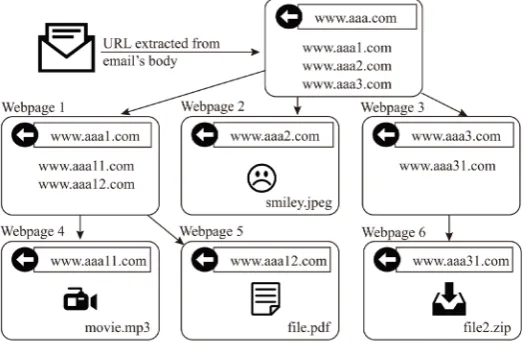
Figure 2 illustrates how the maliciousness of URLs in a spam email is analyzed in SPIKE [21]. The URL links in the email are first extracted from a double-bounce email and SPIKE downloads the html file and attached materials (e.g., java scripts, pdf, doc files) in the entrance page. It then continues to find other URLs in the downloaded pages again. This process is conducted recursively by crawling the linked websites, and all the downloaded materials are analyzed. Emails that are only link to a normal webpage with non-malicious contents are considered as non-malicious spam emails (i.e., all contents of Webpage 1 - 6 in Figure 2 are normal), whereas the emails with at least one suspicious content (i.e., one of Webpage 1 - 6 in Figure 2 is malicious) are identified as malicious spam emails.

3.3. Text Processing and Feature Transformation

In order for the classifier to carry out the classification task effectively, the classifier requires instances as the input instead of the raw spam emails for the learning purpose. The instances consist of informative features with a fixed-length which are extracted from the emails. Thus, appropriate pre-processing steps are required so that the arbitrary data of text messages are transformed into features with numerical features. Figure 1(b) demons- trates the pre-processing module of the spam email detection system. Feature extraction of spam emails involves tokenizing and lemmatizing the documents into bag-of-words (BoW). Tokenization breaks the sentences in the emails into pieces of words and removes frequent words called stop words such as “the”, “which”, “are”, etc. Besides filtering out stop words, lemmatization also reduces the number of words in BoW by transforming redundant words that end with “ing”, “ed” and “s” into their root word (e.g., “learned” to “learn”).

The BoW features usually consist thousands or millions of feature vectors. In general, only some features are informative and are able to differentiate different classes. Therefore, feature selection is carried out to select the most informative features in order to reduce the number of dimensions and avoid the computational complexity. Firstly, the initial training data are transformed into feature vectors with term frequency-inverse document fre-

quency (TF-IDF) feature representation. Next, linear ₁ Support Vector Machines (SVM) is used as a feature selection strategy that requires two steps; training using linear SVM [22] and eliminating features with low weights [23]. SVM is able to find a decision boundary by optimizing the following objective function:

( )

(

)

2 , =1 T 1 min 2

s.t. 1 , 1, ,

0, 1, , .

m

i b

i

i i i

i

C

y b i m

i m ξ φ ξ ξ + + ≤ − = ≤ =

∑

  w w

w x (10)

which maximizes the margin w 2 of hyperplane wT

φ

( )

xi +b between two classes yi∈ ±1 and contains

only a minimum training error ξ_i (i.e., training data located above the support vectors which belong to the class of the training data). The parameter C controls the trade off between margin maximization and errors of the SVM on training data, where a larger C corresponds to a higher penalty to errors. The weights

w

obtained is used to select N_f number of features by choosing the highest N_f-rank weights.

To represent the selected features of initial training data and the remaining training data, the normalized TF-IDF [24] is used to measure the importance of a word to a document (i.e., document refers to the spam email) in the collection of documents given by the following equation:

(

)

( )

_{( )}

_{

_}

TF-IDF , , log

1 : d d t D f t

t d D

f t d D t d

 

= × _ _

+ ∈ ∈

 

∑

(11)

where f_d

( )

t , _d

( )

t f t

∑

, D and

{

d∈D t: ∈d

}

are the frequency of term t in a document d, the total frequencies of all terms in document d, the total number of document in corpus and number of documents which have term t, respectively. The normalized term frequency (TF) is used to provide a balanced value to all documents that have a different number of words. If term t appears frequently in a document d_i and seldom occurs in other documents in D, the value of TF-IDF would be high where both TF and inverse document frequency (IDF) obtain high values. This indicates that term t is important to document d_i. Otherwise, if either the occurrence of term t is low in document d_i or term t is always appears in other documents in D, this would indicate that term t is not important to document d_i where the value of TF-IDF is low or “0”.

After going through the entire procedure above, these data are used as the input to the classifier model. The details of the classifier model are discussed in the previous Section 2.2.

3.4. Outlier Detection

Although SPIKE can judge the maliciousness of spam emails, the analysis takes time, from a few minutes to even longer than ten minutes. Therefore, it is difficult to check all the collected double-bounce emails by SPIKE in real time. We introduce the outlier detection mechanism into RAN-LSH in order to reduce the number of spam emails to be checked by SPIKE. That is, only a new type of unknown spam emails (i.e., outlier) should be selected and sent to SPIKE for labeling. For this purpose, we propose a spam email detection system by combining RAN-LSH classifier [15] and SPIKE, so that the learning time is accelerated compared to when using SPIKE alone. In this study, we detect an outlier based on the output margin θ_m, outlier threshold θ_o and the occurrence frequency threshold θ_N. The data with low output margins are considered as unknown emails for the current classifier and thus should be categorized as outlier. In addition, the number of similar data in each entry N_e is also important to decide whether the data is outlier or not. We assume that the data that do not frequently occurred (i.e., data allocated to an entry with small N_e) can also be categorized as outlier although the output margins are slightly higher than θ_m. The outlier flag F_eO is calculated using Equation (6). The algorithm of the outlier detection is summarized inAlgorithm 4.

4. Performance Evaluation

4.1. Experimental Setup

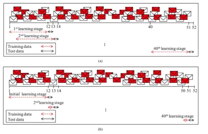
In the former experiment, we investigate the effects of the following three threshold parameters to the perfor- mance: threshold of accumulation ratio θ_a, that of output margin θ_m, and that of tolerant distance θ_p. In the latter experiment, we study the effect of incremental learning through comparison with the batch learning scheme. Figure 3 illustrates how labeled spam emails are trained in (a) batch learning scheme and (b) incremen- tal learning scheme. In the batch learning scheme, we adopt the conventional RBF network (RBFN) (i.e., RBFN usually used as batch learning [25]) as a classifier and a sliding window is introduced to define a data set to be trained every day. In this experiment, the time-window size is preliminarily determined as 12 days via the cross- validation using the spam emails collected during a different period. Therefore, as seen inFigure 3(a), the first learning stage is carried out on Day 12 using a set of spam emails collected from Day 1 to Day 12, and the data set from Day 13 is used to test the performance. Then, the time-window is shifted by one day at the second learning stage; that is, a set of spam emails collected from Day 2 to Day 13 is used for training, and the data set from Day 14 is used to test. Note that RBFN is retrained with a set of 12-day spam emails at every learning stage in a batch mode. On the other hand, in the incremental learning scheme, batch learning is first applied to an initial data set, which is composed of spam emails collected in the first 12 days. After that, this initial detection model is updated daily using one day training data and the system is tested using the next day data. A set of spam emails collected is forwarded to SPIKE to get the labels on maliciousness, and the pairs of a spam email and its class label are used as a training set on the next day. The number of collected spam emails is different every day. Their maximum, minimum, and average numbers are 756, 26, and 207, respectively.

In this detection system, three parameters are determined empirically. The parameters are accumulation ratio

a

θ , output margin θ_m and tolerant distance θ_p. In the following experiment, the parameters are set to:

0.9

a

θ = , θ =m 0.2, and θ =p 2. Meanwhile, the error threshold

ε

is set to 0.5. The other parameters, RBF

width

σ

, the number of partitions P, errors penalty of SVM C, outlier threshold θ_o, occurrence frequency threshold θ_N and time-window size are determined in the initial learning phase through the cross-validation. There are 20,448 double bounce emails with 8334 malicious spam emails and 12,114 non-malicious spam emails used in this study that were collected from 1st March 2013 to 10th May 2013.

(a)

[image:11.595.95.515.81.351.2]

(b)

Figure 3. Comparison of learning scheme between batch learning and incremental learning. (a) Batch learning; (b) Incremental learning.

However, if the malicious spam email detection system is able to obtain high rate of both recall and precision, we can say that the developed system is nearly a perfect detection system.

4.2. Effects of Threshold Parameters

First, let us examine the threshold parameters and their effect to the detection system. Here, we study the influence of θ_a, θ_m and θ_p so that the parameters are optimized to ensure fast learning property of the detection system while having low misclassification rate. The first parameter is the threshold of accumulation ratio θ_a. If θ_a is set to a large value, an eigenspace to define hash functions has high-dimensions. Thus, the length of a hash code becomes long, resulting in the enlargement of a hash table. Therefore the searching of similar data would require a longer time since there are many hash values registered in hash table. The next parameter is the output margin threshold θ_m. This parameter controls the amount of selected data to be learned by RAN-LSH. As the value of θ_m is set to a higher value, the representation of the “not well-learned” region would become wider and the number of selected data is increased in the incremental learning phase, resulting in slower learning. The third important parameter is the tolerant distance θ_p which determines the distance of near RBF bases. By updating the weights of only near RBF bases (i.e., using small value of θ_p), the time needed to solve the linear equation using Singular Value Decomposition (SVD) is shorten, thus the learning time would be accelerated.

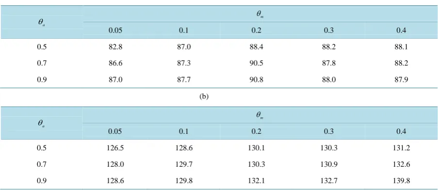
To determine an appropriate value of each parameter, the cross-validation is performed for the initial training set, and the obtained parameter values are fixed over the incremental phase. Table 1(a)and Table 1(b)show the F1 measure and the learning time, respectively, using several combination values of the accumulation ratio θ_a and output margin θ_m. As seen in Table 1(a), the highest F1 measure is obtained when θ =a 0.9 and

0.2

m

θ = . For output margin θ ≤m 0.2, F1 measure does not differ much from the F1 measure with output

margin θ =m 0.2. This result is not surprising because high value of output margins represents that the data are

[image:12.595.87.539.125.321.2]

Table 1. The evaluation using several values of accumulation ratio θ_a and output margin threshold θ_m for the spam email detection system. The performance measures are: (a) the F1 measure [%], and (b) initial learning time [sec.].

(a)

a

θ θm

0.05 0.1 0.2 0.3 0.4

0.5 82.8 87.0 88.4 88.2 88.1

0.7 86.6 87.3 90.5 87.8 88.2

0.9 87.0 87.7 90.8 88.0 87.9

(b)

a

θ θm

0.05 0.1 0.2 0.3 0.4

0.5 126.5 128.6 130.1 130.3 131.2

0.7 128.0 129.7 130.3 130.9 132.6

0.9 128.6 129.8 132.1 132.7 139.8

Therefore, the output margins θ_m can be estimated to be between “0” to “0.2” where the data with output margins in these range are important to be learned to reduce the misclassification rate.

On the other hand, Table 2 demonstrates the suitable value of the tolerant distance θ_p using appropriate value of θ_a and θ_m obtained previously which are “0.9” and “0.2”, respectively. Tolerant distance θ_p also give influence to the classification rate and the speed of the detection system by controlling the distance which defines the area of near RBF bases. As we can see, the suitable value for the tolerant distance is 2. It means that only the RBF centers that differ from the given training data at two projection vector v_i are used to update the weight. If the θ_p is too small, it indicates that the area of selected RBF bases is not enough to approximate the weights correctly. Whereas for θ_p that is too large, it would be similar to the approach of updating weights using all RBF bases. Thus, the size of RBF outputs Φ in ΦW D= would be bigger and therefore, the decomposition steps using SVD would require a longer time. Even though the results show the evaluation performance during initial learning, we expect a similar result from the incremental learning phase. It is because parameter θ_a, θ_m and θ_p are also required during the incremental learning phase. For the next experiment, we set the value of θ_a, θ_m and θ_p to be “0.2”, “0.9” and “2”, respectively.

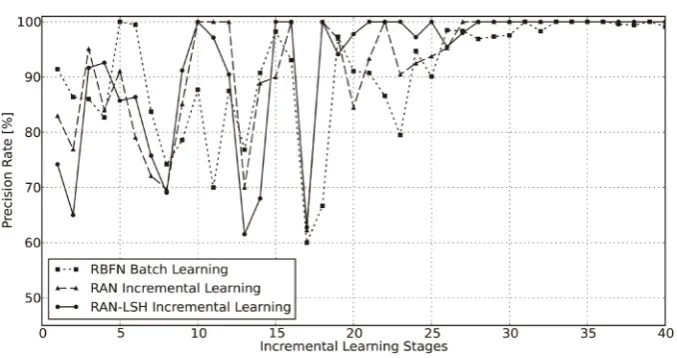
4.3. Effectiveness of Incremental Learning

All learning parts in the detection system including pre-processing and classifier module are very crucial which give effect to the performance result. In this experiment, we compare the performance of the proposed online detection system with different learning scheme and classifier model to see the competency of the proposed method. Figure 4and Figure 5show the recall rate and precision rate for the detection system with the follow- ing three combinations of classifiers and learning schemes: RBFN (batch learning), RAN (incremental learning), and RAN-LSH (incremental learning) (see Figure 3). The batch learning is carried out using 12-days of training data and it is retrained incrementally. While for the incremental learning, the classifier is updated incrementally using 1-day of training data. As seen in Figure 4 and Figure 5, the proposed one-pass learning of the detection system is capable to learn and carry out the classification task effectively since our proposed system obtained almost the same classification rate as the memory-based learning approach (i.e., batch learning). In fact, our proposed method does not need large memory size to store the training data compared to the memory-based learning. In this study, 12-days length of window size is used for the batch learning to learn incrementally, whereas for incremental learning, only 1-day data set is used as training data. Besides that, we also compare the performance of conventional classifier RAN using the same incremental learning scheme. Our previous study in

[image:13.595.133.467.83.258.2]

Figure 4. Transitions of recall rates in the malicious spam email detection system with three learning schemes.

[image:13.595.130.469.289.468.2]

Figure 5. Transitions of precision in the malicious spam email detection system with three learning schemes.

Table 2. The performance using different values of tolerant distance θ_p.

Evaluation

p θ

0 1 2 5

F1 measure [%] 88.5 88.8 89.3 89.3

Initial learning time [sec.] 138.2 139.1 140.1 144.9

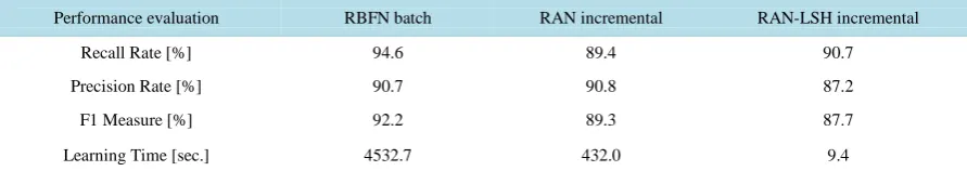
4.4. Overall Performance of Malicious Spam Email Detection System

[image:13.595.86.551.521.593.2]

[image:14.595.92.538.102.181.2]

Table 3. Overall performance of malicious spam email detection system.

Performance evaluation RBFN batch RAN incremental RAN-LSH incremental

Recall Rate [%] 94.6 89.4 90.7

Precision Rate [%] 90.7 90.8 87.2

F1 Measure [%] 92.2 89.3 87.7

Learning Time [sec.] 4532.7 432.0 9.4

the classification rate of recall rate, precision rate and F1 measure do not differ much from the other model, we can conclude that the proposed system is able to update efficiently and able to give class label of the incoming emails within a short time.

5. Conclusions

We have proposed a malicious spam email detection system using BoW features, where the classifier adopts LSH to select essential data and near RBF bases. We use two types of essential data: 1) the data located close to a class boundary; and 2) the data located outside of the learned region (i.e., outlier). The proposed scheme provides desirable learning characteristics as an autonomous malicious spam email detection system and able to adapt to new trends of malicious emails quickly. In addition, our detection system is quite fast compared with SPIKE which often needs a long time to complete the maliciousness analysis. By using the proposed system, it is possible to give proper alerts to users quickly based on up to date information. Since the learning is quite fast and the detection performance is comparable to the conventional models, we can conclude that the proposed system is suitable to be implemented in an email client software on the user side.

Currently, the proposed detection system has no pruning function for RBF bases. Therefore, as the learning is continued for a long time, the number of RBF could be increased excessively, and this causes longer learning time. Then, in the worst scenario, the learning may not converge before new training data are given. To avoid such a disastrous situation, a proper number of RBF bases should always be maintained by introducing an online pruning mechanism into RAN-LSH. Besides that, our detection system uses selected features from initial learning training data. As our future work, we intend to construct an adaptive hash table to adapt to the changes of feature vectors from the recent BoW without forgetting the previous knowledge. It is expected that the detection system would be more stable and robust to the new malicious spam email attacks.

Acknowledgements

This work is partially supported by the Ministry of Education, Science, Sports and Culture, Grant-in-Aid for Scientific Research (C) 24500173, the University of Tun Hussein Onn Malaysia (UTHM) and the Ministry of Education Malaysia (KPM).

References

[1] Vuong, T.P. and Gan, D. (2012) A Targeted Malicious Email (TME) Attack Tool. 6th International Conference on Cybercrime, Forensics, Education and Training (CFET), Christ Church Canterbury.

[2] Nagarjuna, B.V.R.R. and Sujatha, V. (2013) An Innovative Approach for Detecting Targeted Malicious E-Mail. Inter-national Journal of Application or Innovation in Engineering & Management (IJAIEM), 2, 422-428.

[3] Symantec Corporation (2014) Internet Security Threat Report 2014, Vol. 19, 1-98.

http://www.symantec.com/content/en/us/enterprise/other_resources/b-istr_main_report_v19_21291018.en-us.pdf

[4] Hurcombe, J. (2014) Malicious Links: Spammers Change Malware Delivery Tactics.

http://www.symantec.com/connect/blogs/malicious-links-spammers-change-malware-delivery-tactics

[5] Amin, R.M. (2011) Detecting Targeted Malicious Email through Supervised Classification of Persistent Threat and Recipient Oriented Features. Ph.D. Dissertation, Dept. Eng. and Applied Sciences, George Washington University, Washington.

http://www.researchgate.net/publication/224265677_Detecting_Targeted_Malicious_Email_Using_Persistent_Threat_ and_Recipient_Oriented_Features

[7] Jungsuk, S. (2011) Clustering and Feature Selection Methods for Analyzing Spam Based Attacks. Journal of the Na-tional Institute of Information and Communications Technology, 58, 35-50.

[8] Criddle, L. What Are Bots, Botnets and Zombies?

http://www.webroot.com/za/en/home/resources/tips/pc-security/security-what-are-bots-botnets-and-zombies

[9] Nazirova, S. (2011) Survey on Spam Filtering Techniques. Communications and Network, 3, 153-160.

http://www.scirp.org/journal/PaperInformation.aspx?PaperID=6769#.VPkYAzWlilN

http://dx.doi.org/10.4236/cn.2011.33019

[10] Datar, M., Immorlica, N., Indyk, P. and Mirrokni, V.S. (2004) Locality-Sensitive Hashing Scheme Based on p-Stable Distributions. Proceedings of Symposium on Computational Geometry (SoCG'04), 253-262.

http://dl.acm.org/citation.cfm?id=997857

http://dx.doi.org/10.1145/997817.997857

[11] Andoni, A. and Indyk, P. (2008) Near-Optimal Hashing Algorithms for Approximate Nearest Neighbor in High Di-mensions. Communications of the ACM, 51, 117-122. http://dl.acm.org/citation.cfm?id=1327494

http://dx.doi.org/10.1145/1327452.1327494

[12] Gu, X., Zhang, Y., Zhang, L., Zhang, D. and Li, J. (2013) An Improved Method of Locality Sensitive Hashing for In-dexing Large-Scale and High-Dimensional Features. Signal Processing, 93, 2244-2255.

http://dl.acm.org/citation.cfm?id=2464367

http://dx.doi.org/10.1016/j.sigpro.2012.07.014

[13] Lee, K.M. and Lee, K.M. (2012) Similar Pair Identification Using Locality-Sensitive Hashing Technique. Proceedings of Joint 6th International Conference on Soft Computing and Intelligent Systems (SCIS) and 13th International Sympo-sium on Advanced Intelligent Systems (ISIS), 2117-2119.

http://ieeexplore.ieee.org/xpl/freeabs_all.jsp?arnumber=6505385

http://dx.doi.org/10.1109/SCIS-ISIS.2012.6505385

[14] Shen, H., Li, T., Li, Z. and Ching, F. (2008) Locality Sensitive Hashing Based Searching Scheme for a Massive Data-base. Proceedings of IEEE Southeastcon’08, 123-128.

http://ieeexplore.ieee.org/xpl/freeabs_all.jsp?arnumber=4494271

[15] Ali, S.H.A., Fukase, K. and Ozawa, S. (2013) A Neural Network Model for Large-Scale Stream Data Learning Using Locally Sensitive Hashing. Neural Information Processing Lecture Notes in Computer Science, 369-376.

http://link.springer.com/chapter/10.1007%2F978-3-642-42054-2_46

[16] Platt, J. (1991) A Resource-Allocating Network for Function Interpolation. Neural Computation, 3, 213-225.

http://sci2s.ugr.es/keel/pdf/algorithm/articulo/plat1991.pdf

http://dx.doi.org/10.1162/neco.1991.3.2.213

[17] Ozawa, S., Pang, S. and Kasabov, N. (2008) Incremental Learning of Chunk Data for Online Pattern Classification Systems. IEEE Transactions on Neural Networks, 19, 1061-1074. http://www.lib.kobe-u.ac.jp/repository/90001005.pdf

http://dx.doi.org/10.1109/TNN.2007.2000059

[18] Haykin, S. (1999) Neural Networks: A Comprehensive Foundation. Prentice Hall, Upper Saddle River.

[19] Langley, P. (1994) Selection of Relevant Features in Machine Learning. Proceedings of the AAAI Fall Symposium on Relevance, New Orleans, 4-6 November 1994, 140-144.

[20] Oyang, Y.J., Hwang, S.C., Ou, Y.Y., Chen, C.Y. and Chen, Z.W. (2005) Data Classification with Radial Basis Func-tion Networks Based on a Novel Kernel Density EstimaFunc-tion Algorithm. IEEE Transactions on Neural Networks, 16, 225-236. http://dx.doi.org/10.1109/TNN.2004.836229

http://ieeexplore.ieee.org/xpl/abstractAuthors.jsp?tp=&arnumber=1388471&url=http%3A%2F%2Fieeexplore.ieee.org %2Fiel5%2F72%2F30214%2F01388471.pdf%3Farnumber%3D1388471

[21] Dai, Y., Tada, S., Ban, T., Nakazato, J., Shimamura, J. and Ozawa, S. (2014) Detecting Malicious Spam Mails: An On-line Machine Learning Approach. Neural Information Processing Lecture Notes in Computer Science, 8836, 365-372.

http://link.springer.com/chapter/10.1007%2F978-3-319-12643-2_45

[22] Cortes, C. and Vapnik, V. (1995) Support-Vector Networks. Machine Learning, 20, 273-297.

http://link.springer.com/article/10.1023%2FA%3A1022627411411

http://dx.doi.org/10.1007/BF00994018

[23] Brank, J., Grobelnik, M., Milić-Frayling, N. and Mladenić, D. (2002) Feature Selection Using Linear Support Vector Machines. Proceedings of the 3rd International Conference on Data Mining Methods and Databases for Engineering,

Finance, and Other Fields, Bologna, Italy, 25-27 September 2002, 84-89.

[25] Ozawa, S., Tabuchi, T., Nakasaka, S. and Roy, A. (2010) An Autonomous Incremental Learning Algorithm for Radial Basis Function Networks. Journal of Intelligent Learning Systems and Applications, 2, 179-189.

http://www.scirp.org/journal/PaperInformation.aspx?PaperID=3333#.VPkOYTWlilM