Munich Personal RePEc Archive
Determinants of Suicides in Denmark:
Evidence from Time Series Data
Halicioglu, Ferda and Andrés, Antonio R.
Yeditepe University
2010
Online at
https://mpra.ub.uni-muenchen.de/24980/
Determinants of Suicides in Denmark: Evidence from Time Series Data
Abstract
This research examines empirically the determinants of suicides in Denmark over the period 1970-2006. To our knowledge, there exist no previous study that estimates a dynamic econometric model of suicides on the basis of time series data and cointegration framework at disaggregate level. Our results indicate that suicide is associated with a range of socio-economic factors but the strength of the association can differ by gender. In particular, we find that a rise in real per capita income and fertility rate decreases suicides for males and females. Divorce is positively associated with suicides and this effect seems to be stronger for men. A fall in unemployment rates seems to lower significantly suicides in males and females. Policy implications of suicides are discussed with some appropriate recommendations.
Keywords: Suicide, Denmark, Time Series, Cointegration
Correspondence to:
Ferda Halicioglu
Corresponding Author
Department of Economics, Yeditepe University, Istanbul,
34755 Turkey
Antonio R. Andrés
Co-author
Institute of Public Health
Department of Health Services Research Bartholins Allé 1, Building 1264
Aarhus University 8000 Aarhus C, Denmark
1. Introduction
There are several reasons to be interested in the determinants of societal suicide rates. First,
suicide is a major public health issue in many Western countries. According to the World
Health Organization (WHO) [1], in 2004 suicide was responsible for 1.3% of the total burden
of disease worldwide and for 2% of the burden in the European region. Second, in addition to
its heavy economic costs1, suicide has massive negative effects-psychological pain and
suffering-on the suicide’s family. Third, suicide rates can be considered as a more objective
and reliable indicator of well-being or quality of life than self-reported health measures [2].
Moreover, suicide rates do not have the common problems associated with survey data on
self-reported well-being (i.e., cognitive factors that affect subjective responses, such as the
ordering of questions, the wording of the survey, etc.)2. Bertrand and Mullainathan make the
point that in this context that respondents tend to overestimate their subjective well-being and
that socio-economic status affects the way people respond to a survey. Self-reported measures
are often challenged on the basis of reliability and validity. Finally, it has also been shown
that there is a strong correlation between suicide and subjective well-being at the individual as
well at the aggregate level [3], [2]. Recently, a study using American data concluded that the
determinants of well-being are the determinants of suicide [4].
Generally, national wealth and quality of life have a positive correlation. That is, richer
nations have better quality of life. Nevertheless, it is remarkable that wealthy countries also
have higher suicide rates than poor countries. The explanation for this is likely to be a
1
complex mixture of socio-economic factors. This article is a first attempt to understand the
Danish suicide problem better. The suicide rate in Denmark was among the highest in Europe
in 1980, and, even though suicide rates have declined for both men and women and for almost
all age groups since then, Denmark still has higher suicide rates than other countries in
Scandinavia [8].
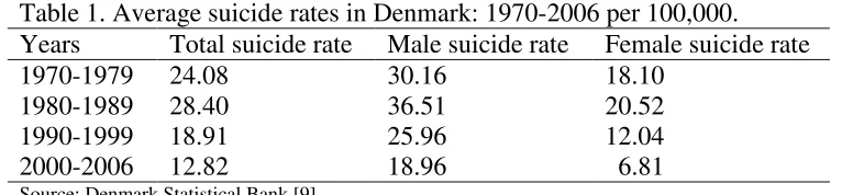
Table 1 displays the average male and female suicide rates for the study period 1970-2006.
Male suicide rates are higher than female rates. Specifically, average suicide rates for males
are two times higher than for females. There has also been a decline in reported suicide rates
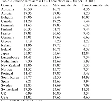
over the study period. Reported suicide rates vary considerably across the Organization for
Economic Cooperation and Development (OECD), as Table 2 shows. In 2004 the highest
suicide rate was reported by Japan (24.97 per 100,000 people) followed by South Korea
(23.77 per 100,000 people). Greece had the lowest suicide rate at 3.19 per 100,000 people.
For male suicide rates, Japan ranked the highest among 23 OECD countries. For female
suicide rates, South Korea was the highest in 2004. Across all countries, men are three times
[image:4.595.62.445.514.603.2]more likely to die due to suicide than women.
Table 1. Average suicide rates in Denmark: 1970-2006 per 100,000. Years Total suicide rate Male suicide rate Female suicide rate
1970-1979 24.08 30.16 18.10
1980-1989 28.40 36.51 20.52
1990-1999 18.91 25.96 12.04
2000-2006 12.82 18.96 6.81
Table 2. Suicide rates across OECD countries in 2004 per 100,000.
Country Total suicide rate Male suicide rate Female suicide rate
Australia 10.50 16.71 4.36
Austria 17.35 27.03 8.20
Belgium 19.06 28.44 10.07
Canada 11.29 17.26 5.44
Denmark 11.65 17.03 6.38
Finland 20.33 31.71 9.44
France 17.81 26.65 9.45
Germany 13.01 19.68 6.63
Greece 3.19 5.20 1.22
Iceland 11.96 17.72 6.17
Ireland 10.51 16.71 4.38
Japan 23.97 35.64 12.84
Luxembourg 14.41 21.64 7.34
Netherlands 9.30 12.69 5.98
New Zealand 12.06 19.07 5.33
Norway 11.52 15.77 7.34
Portugal 11.47 17.87 5.48
South Korea 23.77 32.50 14.98
Spain 8.21 12.63 3.94
Sweden 12.83 18.69 7.08
Switzerland 17.36 23.68 11.31
UK 6.99 10.80 3.34
USA 11.02 17.65 4.60
Source: WHO Mortality Database [10]
This paper is novel in many ways. To the best of our knowledge, there is no empirical study
which deals with the issue of suicide from a macro perspective in Denmark that has employed
dynamic econometric models such as the Autoregressive Distributed Lag (ARDL) model3.
Second, in addition to modeling the total number of suicides, we also estimate separate
models for males and females, as the determinants of suicide might differ between sexes.
Understanding gender differences might be important in informing appropriate health
policies. This paper is organized as follows: in the following section, we present a brief
summary of previous research. Next, we describe our empirical model and methodological
approach. Subsequently, we present our empirical findings, followed by the conclusion.
2. Literature review
As indicated elsewhere [12], two of the most frequently employed approaches to the study of
suicide are the sociological approach [13] employed by Durkheim and the economic approach
[14] of Hamermesh and Soss. According to the economic theory of suicide, an individual
decides to commit suicide when the discounted expected lifetime utility remaining to him falls
below some threshold level. This model predicts that suicide rates would increase with age
and unemployment and decrease with income [14].
According to the economic model of suicide, the higher future expected income is, the higher
is the expected utility; thus, living is relatively more attractive than committing suicide, and a
higher income should lower suicide rates. However, Durkheim postulates that higher income
levels increase independence (the opposite of social integration) and might lead to a higher
suicide rate. Along this line Refs. [15, 16] state that economic development increases rates of
suicide. Both the existing economic and sociological theories are inconsistent, and they do not
permit a determination of whether income or economic growth may have a positive or
negative effect on suicide. Durkheim suggests that changes in income are more likely to be
relevant for suicide than the level of income. The empirical evidence for the effect of income
on suicide is mixed, however. Though some empirical studies indicate that suicide rates have
a positive association with income [17-19], there are many others suggesting the opposite
effect [2, 20-26]. Others have reported an insignificant effect of income on suicide [27], [28].
The significant negative correlation effect seems to be stronger for men than for women [11].
Another economic variable that has received a lot of attention is the unemployment rate.
and therefore increasing the likelihood of a person’s committing suicide. The unemployment
rate is often used as a proxy variable for economic hardships and lifetime earnings, because
measuring an person’s agent’s lifetime income is not easy in practice [29]. But unemployment
might be also associated with factors such as depressive episodes, anxiety, and loss of
self-confidence that might lead directly to suicide. The empirical findings are fairly mixed. Much
of the empirical literature reports a positive relationship, associating higher unemployment
with higher suicide rates [21], [27], [23], [24], [30], [20], [29], [25]. Furthermore, the impact
of unemployment might also differ across gender. In particular, male suicide rates are
significantly affected by unemployment, but female suicide rates are not [23].
The seminal work of Durkheim [13] indicates that suicide is influenced by other factors.
These factors relate to the way in which individuals are integrated into a social group that is
regulated by norms and conventions. The sociological perspective of suicide [13] predicts that
lower levels of social integration and regulation are associated with higher societal suicide
rates. From this perspective divorce and fertility rates can be viewed as indicators of social
integration. Divorcecan be a traumatic event for the individuals involved as well as for other
affected parties, and it might lead individuals toward isolation and reduced poor psychological
well-being. Thus, higher divorce rates might be expected to have a positive correlation with
suicide rates. The empirical literature on suicide reports evidence that divorce is positively
associated with suicide rates [20], [23], [24], [31], [15], [22]. Also, some papers show that the
male suicide rate is more sensitive to divorce than the female suicide rate [29], [20], [32],
[22]. Again, endogeneity concerns are relevant here, as divorce might be related to mental
health problems. It should be also noted that this variable might capture the influence of
diverse societal problems. Durkheimian arguments of social integration [13] suggest that
children promotes social and family ties. By increasing social integration, these factors lower
the likelihood of a person’s committing suicide. Empirical research has documented the
existence of a protective effect of fertility against suicide [20], [22], [24]. However, some
studies [33], [34] show that birth rate has either a positive impact or no impact on suicide
rates. One possible explanation for the latter result is that childcare may put excessive strain
on a parent or be too much of an economic burden, thus leading to suicidal behavior [33].
Lastly, the gender differences in suicide represent a double puzzle: while rates of suicide are
far higher among males, females have higher rates of non-fatal attempts. This suggests that
there may be different responses by males and females to the control variables used in the
formal analysis. In light of the gender differential in suicidal behaviour [26], [25], [20], [32],
we run separate models for males and females.
In sum, the formal literature provides ambiguous results on the ways socio-economic factors
relate to male and female suicide rates. Of all the variables considered, the results
corresponding to social factors such as divorce and fertility seem to be more robust than those
related to economic factors such as unemployment and income. Suicide is a very complex
event affected by many variables, many of which we are not able to observe in our sample.
Nonetheless, the variables included here appear to be among the relatively important
determinants.
Following the empirical literature on suicide (for an extensive review of the literature, see
Ref. [35]), we form the following long-run relationship between suicide, income,
unemployment, divorce, and fertility in linear logarithmic form as:
t t t t t
tj a ay au ad a f
s = 0 + 1 + 2 + 3 + 4 +ε , (1)
where the subscript t indexes time period with t =1970,…,2006; j indexes each suicide with j=
0 (total), 1 (male), and 2 (female); yt is per capita real income; ut is the unemployment; dt is
the divorce rate; ft is the fertility rate; and εt is the classical error term.
Recent advances in econometric literature dictate that the long-run relation in equation (1)
should incorporate the short-run dynamic adjustment process. It is possible to achieve this aim
by expressing equation (1) in an error-correction model [36], known as the Engle-Granger
approach. t t i t m i i i t m i i m i m i m i i t i i t i j i t j i j
t b b s b y b u b d b f
s = + ∆ + ∆ + ∆ + ∆ + ∆ +γε +µ
∆ − − = − = = = = − − − 1 5 0 6 4 0 4 1 1 2 0 3 0 3 2 , , 1 0
, , (2)
where ∆ represents change , γ is the speed of adjustment parameter, and εt−1 is the lagged
error term, which is estimated from the residuals of equation (1). The Engle-Granger method
requires that all variables in equation (1) are integrated of order one, I(1), and that the lagged
error term is integrated order of zero, I(0), in order to establish a cointegration relationship. If
some variables in equation (1) are non-stationary, we may use a new cointegration method
[37]. This procedure is known as ARDL approach to cointegration of Pesaran et al. that
its equivalent from equation (1). εt−1 is substituted by linear combination of the lagged
variables as in equation (3):
t t t t t j t i t n i i i t n i i n i n i n i i t i i t i j i t j i j t v f c d c u c y c s c f c d c u c y c s c c s + + + + + + ∆ + ∆ + ∆ + ∆ + ∆ + = ∆ − − − − − − = − = = = = − − − 1 10 1 9 1 8 1 7 , 1 6 5 0 5 4 0 4 1 1 2 0 3 0 3 2 , , 1 0 , (3)
To obtain equation (3), one has to solve equation (1) for εt and lag the solution equation by
one period. Then, this solution is substituted for εt−1 in equation (2) to arrive at equation (3).
Equation (3) is a representation of the ARDL approach to cointegration.
The bounds-testing procedure is based on the F- or Wald-statistics, and this is the first stage of
the ARDL cointegration method. Accordingly, a joint significance test that implies no
cointegration hypothesis, (H0: c6 =...=c10 =0), against the alternative hypothesis, (H1: at
least one c6 toc10 ≠0), should be performed for equation (3). The F-test used for this
procedure has a non-standard distribution. Thus, Pesaran et al. compute two sets of critical
values for a given significance level with and without a time trend. One set assumes that all
variables are I(0), and the other set assumes that they are all I(1). If the computed F-statistic
exceeds the upper critical bounds value, then the H0 is rejected. If the F-statistic falls into the
bounds, then the test becomes inconclusive. Lastly, if the F-statistic is below the lower critical
bounds value, it implies no cointegration. Given the size of the sample used in this study (37
observations), the critical values for the bounds F-test reported by Ref. [38] are more
Once a long-run relationship has been established, equation (3) is estimated using an
appropriate lag-selection criterion. At the second stage of the ARDL cointegration procedure,
it is also possible to obtain the ARDL representation of the error-correction model. To
estimate the speed with which the dependent variable adjusts to independent variables within
the bounds-testing approach, following Pesaran et al., the lagged-level variables in equation
(3) are replaced by ECt-1 as in equation (4):
t t i t k i i i t k i i k i k i k i i t i i t i j i t j i j
t s y u d f EC
s =α + α ∆ + α ∆ + α ∆ + α ∆ + α ∆ +λ +µ
∆ − − = − = = = = − − − 1 5 0 5 4 0 4 1 1 2 0 3 0 3 2 , , 1 0
. . (4)
A negative and statistically significant estimation of λ not only represents the speed of
adjustment but also provides an alternative means of supporting cointegration between the
variables. Annual data over the period 1970-2006 were used to estimate equation (3) by the
ARDL cointegration procedure of Pesaran et al. All data have been collected on-line from
Statistics Denmark [9].
The time-series properties of the variables included in equation (1) are checked through
Augmented Dickey-Fuller (ADF) [39] to make sure that the variables in consideration are not
integrated at an order higher than one, I(1). The critical values of Refs [37, 38] are not
applicable in the presence of I(2) variables. The results of the ADF tests are reported in Table
3. The variables of per capita real income (yt) and fertility rate (ft) are stationary in their
levels, whereas other variables contain a unit root in their levels which warrant our applying
the bounds-testing procedure. Visual inspection of the variables in logarithms indicated to us
Table 3. Tests for integrationa. ADF test statistic
Variable Levels k lag 1st
Differences
k lag
0 , t
s -2.2498 1 -3.5906* 1
1 , t
s -2.3817 1 -4.6671* 1
2 , t
s -2.0785 1 -4.0421* 1
t
y 3.6275* 3 -4.6035* 4
t
u -1.3618 2 -2.9852* 3
t
d -2.4867 1 -3.3425* 1
t
f -5.0959* 4 -2.5101 1
a
Sample levels 1976-2006 and differences 1977-2006. Rejection of unit root hypothesis, according to McKinnon’s [40] critical value at 5% is indicated with an asterisk. ADF tests include an intercept and a 1 to 5 lagged difference variable and k stands for the lag level that maximizes the AIC (Akaike Information Criteria). The critical values are -3.5615 and -2.9627 at levels and differences, respectively.
Equation (3) is estimated in two stages. In the first stage of the ARDL procedure, the long-run
relationship of equation (1) was established in two steps. First, the order of lags on the
first-differenced variables for equation (3) was obtained from unrestricted Vector Auto Regression
(VAR) by means of Akaike Information criteria (AIC) and the Schwarz Bayesian Criterion
(SBC). The results suggest the optimal lag length as 2, but this stage of the results is not
presented here to conserve space. Second, a bound F-test was applied to equation (3) in order
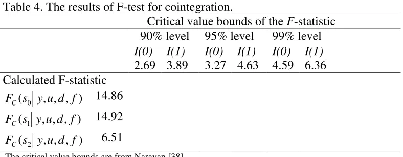
to establish a long-run relationship between the variables. The results of the bounds F-testing
are displayed in Table 4. The results show that total suicides, male suicides, and female
suicides all enter the regression equations as dependent variables in the long-run.
Table 4. The results of F-test for cointegration.
Critical value bounds of the F-statistic 90% level 95% level 99% level
I(0) I(1) I(0) I(1) I(0) I(1)
2.69 3.89 3.27 4.63 4.59 6.36 Calculated F-statistic
) , , , (s0 y u d f
FC 14.86
) , , , (s1 y u d f
FC 14.92
) , , , (s2 y u d f
FC 6.51
[image:12.595.68.462.589.743.2]The ARDL cointegration procedure was implemented to estimate the parameters of equation
(3) with maximum order-of-lag set to 2, which is selected on the basis of SBC and R2
selection criteria. This stage involves estimating the long-run and short-run coefficients of
equations (1) and (2).
4. Results
The summary ARDL results with some diagnostic tests for total suicides, male suicides, and
female suicides are presented in Tables 5-7 respectively. The overall empirical results appear
to be rather satisfactory, considering the small sample size. First, income enters negatively in
the regressions for overall, male, and female suicides. The long-run elasticity of suicide with
respect to income is highest in the case of female suicides. This is -3.22, suggesting that each
1% increase in per capita real income will decrease the number of female suicides by 3.22 %.
The long-run income elasticities for total and male suicides are -2.22 and -1.73, respectively.
This finding implies that females are more vulnerable to income loss than males. Second,
unemployment rates are positively and significantly related to overall, male, and female
suicide rates. The long-run elasticity of suicide with respect to unemployment seems to be
almost the same in all the categories, indicating that a 1% rise in unemployment rates will
trigger an increase in all suicides by about 0.1%. Therefore, it is crystal clear that the impact
of male and female unemployment on suicides is identical. Gender seems to have no special
effect on a suicide decision, when an individual becomes unemployed. Third, divorce rates
are positively correlated with suicide rates but are statistically insignificant. Finally, we find a
negative association between fertility rates and suicide rates. In the case of female suicides, a
almost halved in the case of male suicides, suggesting that females are naturally more
protective of their families.
The long-run elasticity of suicide with respect to the fertility rate variable implies that a 1%
increase in fertility will decrease total suicides by 0.70% and female suicides by 0.92% but
male suicides by only 0.57%. In regards to the relative magnitude of the explanatory variables
in this study, the fertility rate seems to be the second most important factor in explaining the
suicide rates, followed by divorce and unemployment rates.
All the error correction terms in the estimated models are statistically significant and with the
expected signs. They also represent a strong level of dynamic equilibrium between the
Table 5. ARDL cointegration results. Panel A.
Estimated long-run coefficients using the ARDL approach for aggregate suicide model: ARDL (1,0,2,0,2) selected based on the Schwarz Bayesian Criterion, 1970-2006.
Dependent variable st,0
Regressor Coefficient Standard error T-ratio
t
y -2.2215* 0.1407 15.7441
t
u 0.1051* 0.0409 2.5707
t
d 0.3447 0.4309 0.7999
t
f -0.7003** 0.3352 2.0891
Panel B.
Error correction representation results. Dependent variable∆st,0
Regressor Coefficient Standard error T-ratio
t y
∆ -1.4483* 0.3118 4.6449
t u
∆ 0.0560 0.0518 1.0809
t d
∆ 0.2253 0.2877 0.7833
t f
∆ -0.0846 0.3567 0.2373
1 −
t
EC -0.6536* 0.1450 4.5066
Diagnostic tests 2
R 0.45 F-statistic 5.16* χSC2 (1) 5.82 2 (1) FF
χ 0.17
RSS 0.06 DW-statistic 2.18 2(2) N
χ 2.99 2(1)
H
χ 0.81
*
Table 6. ARDL cointegration results. Panel A.
Estimated long-run coefficients using the ARDL approach for male suicide model: ARDL (1,0,2,1,2) selected based on the R-Bar Squared Criterion, 1970-2006.
Dependent variable st,1
Regressor Coefficient Standard error T-ratio
t
y -1.7295* 0.1446 11.9539
t
u 0.0970** 0.0426 2.2746
t
d 0.3282 0.4866 0.6745
t
f -0.5794 0.3527 1.6425
Panel B.
Error correction representation results
Dependent variable∆st,1
Regressor Coefficient Standard error T-ratio
t y
∆ -1.2706* 0.2649 4.7948
t u
∆ 0.0695 0.0612 1.1371
t d
∆ 0.5815 0.3592 1.6187
t f
∆ -0.2139 0.3991 0.5360
1 −
t
EC -0.7346* 0.1576 4.6598
Diagnostic tests 2
R 0.48 F-statistic 5.96* χSC2 (1) 6.4871 (1) 2 FF
χ 0.0077
RSS 0.07 DW-statistic 2.60 2(2) N
χ 1.9560 2(1) H
χ 1.2618
*
Table 7. ARDL cointegration results. Panel A.
Estimated long-run coefficients using the ARDL approach for female suicide model: ARDL (1,2,1,2,2) selected based on the R-Bar Squared Criterion, 1970-2006.
Dependent variable st,2
Regressor Coefficient Standard error T-ratio
t
y -3.2146* 0.1785 18.0085
t
u 0.0958*** 0.0543 1.7628
t
d 0.1636 0.6366 0.2570
t
f -0.9219** 2.5769 2.0300
Panel B.
Error correction representation results. Dependent variable∆st,2
Regressor Coefficient Standard error T-ratio
t y
∆ -4.5916* 1.2742 3.6036
t u
∆ -0.2036 0.1221 1.6665
t d
∆ 0.2473 0.5354 0.4619
t f
∆ 1.0567*** 0.5973 1.7690
1 −
t
EC -0.7509* 0.1510 4.9721
Diagnostic tests 2
R 0.40 F-statistic 4.38** χSC2 (1) 8.7367 2 (1) FF
χ 0.0090
RSS 0.12 DW-statistic 2.67 2(2) N
χ 3.2717 2(1) H
χ 5.9284
*
, **, and *** indicate, 1%, 5% and 10% significance levels respectively. RSS stands for residual sum of squares. T-ratios are in absolute values.χSC2 , χFF2 , χN2, and χH2 are Lagrange multiplier statistics for tests of residual correlation, functional form mis-specification, non-normal errors and heteroskedasticity respectively. These statistics are distributed as chi-squared variates with degrees of freedom in parentheses. The critical values for χ2(1)=3.84 and χ2(2)=5.99 are at 5% significance level.
5.Discussion
This paper has investigated the determinants of suicides over the period 1970-2006 in
Denmark from a macro perspective, using the bounds approach to cointegration developed by
Pesaran et al. A number of findings have been presented here. Income does significantly
affect suicide rates. In particular, higher income is associated with higher suicide rates. The
direction of this effect is consistent with other studies [21, 22]. According to the economic
committing suicide. This effect seems to be gender specific. The existing empirical evidence
using individual-level data for Denmark suggests that men are more vulnerable than women
to economic conditions [11], but this study reveals contradictory results. Our finding that
unemployment increases suicide rates is in accordance with several empirical studies using
aggregate data [20, 24], among others. Nevertheless, this factor results in almost the same
level of impact in both the male and female sectors of the society, although unemployment
might be related to a number of life-style factors of known impact on suicide. The positive
effect of divorce is in accordance with the sociological perspective on suicide [13], which
argues that divorce lowers social integration and entails a rupture of family ties. From this
perspective a society characterized by a high divorce rate is expected to have a higher suicide
rate. In addition, the effect of divorce on suicide depends on sex; the impact of this factor is
twice as great in males as in females. A similar finding was obtained in the Barstad study of
Norway [41], using a time-series approach. In comparison to income as a cause of suicide, the
magnitude of divorce is considerably greater than unemployment but substantially lower than
income. Finally, following Durkheimian arguments of social integration, fertility rates
increase family integration and promote socials ties and are thus expected to lower societal
suicide rates, although this effect seems to be greater for women than for men. This result is
also consistent with past empirical studies [22, 23]. One can argue that the presence of a
young child may increase parents’ feelings of self-worth, possibly due to their experience of
being needed, and the presence of a dependent child may also increase the sense of obligation.
Women are the natural caregivers and the backbone for the raising of families. They should
thus feel emotionally and physically closer to their families than men. This may explain our
Denmark’s social economic environment is similar to that of other Scandinavian countries
and is also similar to many Western European countries. However, one should be cautious
about generalizing the results of this study to other countries with different socio-economic
environments. This paper also sheds light on the time-series properties of the variables
included in empirical analysis of suicide. Close attention needs to be paid to previous results
based on the stationarity assumption of the time-series used in suicide regressions. More
importantly, individuals might respond to changes in socio-economic factors with some delay,
thus a dynamic approach to modelling suicide seems to be more appropriate. National or
international studies of suicide might be plagued of endogeneity problems. Therefore, it is
clear that extreme care should be given to the interpretation of the final conclusions. The
ARDL approach employed in this paper might overcome the problem of endogenous
regressors in suicide equations.
Recommendations for suicide prevention are generally a combination of strategies targeting
high-risk groups and strategies targeting a whole population. The findings of this study reveal
that labour market conditions are related to suicidal behavior. Perhaps the most immediate
application of these findings would be in government, social agency, and employer responses
to the current economic recession, which is likely to produce increased numbers of suicides.
This might also generate considerable pressure on suicide prevention policies. If suicide
increases during recessions, policy makers might want to re-allocate resources from a focus
on one cause of death to another. In bad economic times characterized by high unemployment
rates, specialist advice on dealing with financial problems is also needed to restrain people’s
impulse towards suicide. Training for GPs and other medical service providers including
specialists could also be provided by local government agencies. Government policies should
further economic incentives to raise birth rates, as these policies will reduce the suicide rate.
The planning suicide of prevention policies should consider both macro-economic conditions
and the individual conditions.
References
[1] World Health Organization. Global Burden of Disease Report updated. Geneva; 2004.
[2] Helliwell J. Well being and social capital: does suicide pose a puzzle? Social Indicators
Research 2007;81:455-496.
[3] Koivumaa-Honkanen H, Honkanen R, Viinamki H, Heikkil J, Kaprio J, Koskenvuo M.
Life satisfaction and suicide: a 20-year follow-up study. The American Journal of Psychiatry
2001;158(3):433-459.
[4] Daly M, Wilson DJ. Happiness, unhappiness, and suicide: an empirical assessment.
Journal of European Economic Association 2009;7:539-549.
[5] Kennelly B, Ennis J, O’Shea E. Economic cost of suicide and deliberate self harm, In
Reach out National Strategy for Action on Suicide Prevention 2005-2014. Department of
Health and Children. Ireland. 2005.
[6] McDaid D, Halliday E, McKenzie M, MacLean J, Maxwell M, McCollam A, Platt S,
Woodhouse A. Issues in the economic evaluation of suicide prevention strategies: practical
and methodological challenges. Personal Social Services Research Unit, LSE. London. 2007.
[7] Bertrand M, Mullainathan S. Do people mean what they say? implications for subjective
survey data. American Economic Review 2001;91(2):67-72.
[8] Nordentoft M. Prevention of suicide and attempted suicide in Denmark. Danish Medical
Bulletin 2007;54(4):306-369.
[9] Statistics Denmark (StatBank Denmark), http://www.statbank.dk/; accessed on Feb 15
2010.
[10] World Health Organization. WHO Mortality Database. Last update 16 February 2010.
Geneva. 2010.
[11] Qin P, Agerbo E, Mortensen PB. Suicide risk in relation to socioeconomic, demographic,
psychiatric and familial factors: a national register based study of all suicides in Denmark
[12] Marcotte DE. The economics of suicide, revisited. Southern Economic Journal 2003;
69(3):628-43.
[13] Durkheim E. Suicide: a study in sociology. New York: Free Press; 1951.
[14] Hamermesh DS, Soss NM. An economic theory of suicide. Journal of Political Economy
1974;82 (1):83-98.
[15] Lester D. Patterns of suicide and homicide in the world. New York: Nova Science
Publishers; 1996.
[16] Unnithan NP, Huff-Corzine L, Corzine J, Whitt HP. The currents of lethal violence: an
integrated model of suicide and homicide. Albany: State University of New York Press; 1994.
[17] Hamermesh D. The economics of black suicide. Southern Economic Journal
1974;41:188-199.
[18] Jungeilges J, Kirchgässner G. Economic welfare, civil liberty, and suicide: an empirical
investigation. Journal of Socioeconomics 2002; 31; 215-231.
[19] Viren M. Testing the natural rate of suicide hypothesis. International Journal of Social
Economics 1999;26(12):1428-1440.
[20] Andrés AR. Income inequality, unemployment, and suicide: a panel data analysis of 15
European countries. Applied Economics 2005;3: 439-451.
[21] Brainerd E. Economic reform and mortality in the former Soviet Union: a study of the
suicide epidemic in the 1990s. European Economic Review 2001;45(4-6):1007-19.
[22] Neumayer E. Socioeconomic factors and suicide rates at large-unit aggregate levels: a
comment. Urban Studies 2003;40(13):2769-2776.
[23] Chuang H, Huang W. Regional suicide rates: a pooled cross-section and time-series
analysis. Journal of Socio-Economics 1997;26(3):277-289.
[24] Chuang H, Huang W. A re-examination of the suicide rates in Taiwan. Social Indicators
[25] Minoiu C, Rodríguez A. The effect of public spending on suicide: evidence from US
state data. The Journal of Socio-Economics 2008;37:237-261.
[26] Altinanahtar A, Halicioglu F. A dynamic econometric model of suicide in Turkey.
Journal of Socio-Economics 2009;38:903-907.
[27] Ruhm C. Are recessions good for your health? Quarterly Journal of Economics
2000;115:617-650.
[28] Cuellar AE, Markowitz S. Medicaid policy changes in mental health care and their effect
on mental health outcomes. NBER Working Papers No. 12232. 2006.
[29] Koo J, Cox WM. An economic interpretation of suicide cycles in Japan. Contemporary
Economic Policy 2008;26(1):162-174.
[30] Lin SJ. Unemployment and suicide: panel data analyses. The Social Science Journal
2006;43(4):727-732.
[31] Kunce M, Anderson AL. The impact of socioeconomic factors on state suicide rates: a
methodological note. Urban Studies 2002;39:155-162.
[32] Yamamura E. The different impacts of socioeconomic factors on suicide between males
and females. MPRA Paper 10175, University Library of Munich, 2007.
[33] Chen J, Choi YJ, Mori K, Sawada Y, Sugano S. Socioeconomic studies on suicide: a
survey. CIRJE-f-628 Discussion Papers 2009. The University of Tokyo.
[34] Lester D. Explaining regional differences in suicide rates. Social Science and Medicine
1995;40(5):719-721.
[35] Lester D, Yang B. The economy and suicide: economic perspectives. New York: Nova
Science Publishers; 1997.
[36] Engle RF, Granger CWJ. Cointegration and error correction: representation, estimation,
[37] Pesaran MH, Shin Y, Smith RJ. Bounds testing approaches to the analysis of level
relationships. Journal of Applied Econometrics 2001;16:289-326.
[38] Narayan PK. The saving and investment nexus for China: evidence from cointegration
tests. Applied Economics 2005;37:1979-1990.
[39] Dickey DA, Fuller WA. Likelihood ratio statistics for autoregressive time series with a
unit root. Econometrica1981;49:1057-1072.
[40] McKinnon JG. Critical value for cointegration tests. In: Engel RF, Granger CW, editors.
Long run relationships: readings in cointegration. London: Oxford University Press; 1991.
[41] Barstad A. Explaining changing suicide rates in Norway 1948-2004: the role of social