Munich Personal RePEc Archive
A Quasi-analytical Interpolation Method
for Pricing American Options under
General Multi-dimensional Diffusion
Processes
Li, Minqiang
Georgia Institute of Technology
2009
Online at
https://mpra.ub.uni-muenchen.de/17348/
A Quasi-analytical Interpolation Method for Pricing American Options under General Multi-dimensional Diffusion Processes
Abstract
We present a quasi-analytical method for pricing multi-dimensional American options based on interpolating two arbitrage bounds, along the lines of Johnson (1983). Our method allows for the close examination of the interpolation parameter on a rigorous theoretical footing instead of empirical regression. The method can be adapted to general diffusion processes as long as quick and accurate pricing methods exist for the corresponding European and perpetual American options. The American option price is shown to be approximately equal to an interpolation of two European option prices with the interpolation weight proportional to a perpetual American option. In the Black-Scholes model, our method achieves the same efficiency as Barone-Adesi and Whaley’s (1987) quadratic approximation with our method being generally more accurate for out-of-the-money and long-maturity options. When applied to Heston’s stochastic volatility model, our method is shown to be extremely efficient and fairly accurate.
JEL Classification: C02; C63; G13
I. Introduction
The pricing of American options is one of the oldest problems in finance and its study has attracted experts from various other fields, including mathematics, statistics, economics and operational research. Earliest attempts include McKean (1965), Samuelson (1967), and Merton
(1973). By now, hundreds of papers have been devoted to the study of various aspects of American options. They can be roughly divided into two groups, one focusing more on the
theoretical issues and the other on the computational issues.
Papers focusing on theoretical aspects include: the property of the price function such as
differentiability, convexity, and put-call symmetry (Bergman, Grundy and Wiener (1996), Mc-Donald and Schroder (1998), Shroder (1999)); the property of the critical stock price
bound-ary (van Moerbeke (1976), Barles, Burdeau, Romano and Samsoen (1995), Peskir (2005), Zhu (2006)); different formulations such as partial differential equation with free boundary (McK-ean (1965)), optimal stopping problem and its dual formulation (Bensoussan (1984), Karatzas
(1988), Rogers (2002)), variational inequality (Jaillet, Lamberton and Lapeyre (1990)), and early exercise premium representation (Kim (1990), Jacka (1991), Carr, Jarrow and Myneni (1992));1
convergence and other properties of numerical methods (Lamberton (1993, 1998), Amin and Khanna (1994), Cl´ement, Lamberton, and Protter (2002), Stentoft (2004)); and finally various
generalizations such as general diffusion processes (Detemple and Tian (2002)), multiple under-lying assets (Detemple, Feng and Tian (2003)), and more exotic American-type derivatives (see
Detemple (2006)).
This paper belongs to the second group that looks at the issue of computing American
option prices. By now, more than a dozen well-established pricing methods exist, as well as many others that have not been widely adopted. For a relatively recent but brief survey, see Barone-Adesi (2005). These methods differ in dimensions such as efficiency, accuracy, generality,
robustness, portability to other derivatives or other processes, ease of implementation, etc. In addition to offering a broader menu of pricing methods for practitioners to choose from, the
development of new methods often offers considerable additional insights on various aspects of American options. Because of the huge variety of proposed methods, a clear and unambiguous
classification of all the different methods is difficult. Nonetheless, they can be roughly divided into several somewhat distinctive groups. The first group is the numerical methods based on
solving the valuation partial differential equation. Those include the binomial tree method (Cox, Ross and Rubinstein (1979), Rendleman and Barrter (1979), Curran (1995)), trinomial tree methods and other variations (Parkinson (1977), Breen (1991), Kamrad and Ritchken (1991),
Figlewski and Gao (1999)), finite difference methods (Brennan and Schwartz (1977, 1978), Hull and White (1990)), method of lines (Carr and Faguet (1996)), and penalty method (Khaliqa,
Vossb, and Kazmic (2005)). The second group of methods focuses more on the exercise boundary and usually makes use of the early exercise premium representation. Papers include: Geske and
Johnson (1984), Omberg (1987), Bunch and Johnson (1992), Huang, Subramanyam and Yu (1996), Carr (1998), Ju (1998), Bunch and Johnson (2000), Sullivan (2000), and Kim and Jang
(2008). The third group of methods looks at simulation techniques to value American options, an idea first proposed for European options by Boyle (1977). Examples include Broadie and Glasserman (1997), Longstaff and Schwartz (2001), Moreno and Navas (2003), and Stentoft
(2004)). Numerical techniques such as Richardson extrapolation and variance reduction are often employed in these three groups of methods. Yet a fourth group of methods uses regression
techniques to fit analytical approximations, often based on lower and upper bounds of the American option. These include Johnson (1983), Kim (1994), and Broadie and Detemple (1996).
The final group looks at analytical or quasi-analytical approximations of the American option price, usually by making various approximations to the valuation partial differential equations.
These include MacMillan (1986), Barone-Adesi and Whaley (1987), and Ju and Zhong (1999). In this paper, we develop a new quasi-analytical method which approximates the American
put option price as an interpolation of two bounds. Thus, this paper is very similar in spirit to Johnson (1983) and Broadie and Detemple (1996). In fact, the bounds we use are identical to the ones used in Johnson (1983), except that we formulate our approximation under the framework of
general diffusion processes while Johnson (1983) assumes Black-Scholes model with zero dividend rate. Another important difference is that instead of using a regression procedure as in these two
papers, we work out the interpolation parameter by looking at the partial differential equation the parameter has to satisfy, an idea fruitfully employed in MacMillan (1986), Barone-Adesi
and Whaley (1987), and Ju and Zhong (1999). Our final solution expresses the American put option price as a linear interpolation of two European put option prices, with the interpolation
weight proportional to the price of the perpetual American option. Thus, as long as efficient methods for pricing the European put option and perpetual American option exist, our method can be adapted to general diffusion processes. We first specialize our analysis to the important
case of geometric Brownian motion. In this case, closed-form expressions exist for the European call and perpetual American options. We show that our interpolation method approaches the
correct limits for many limiting cases, most interestingly, as the maturity increases to infinity. The method is then further adapted to one of the leading multi-dimensional models for pricing
derivatives, namely, Heston’s stochastic volatility model. Our method has significant value since the literature is still scarce in terms of pricing American options under this multi-dimensional
In our numerical study, we examine the performance of our method using both short-term, medium-term and long-term options under the geometric Brownian motion model. We select a
broad set of parameter values for the interest rate, dividend rate, volatility, and current stock prices. Our method gives fairly accurate approximations for the critical stock price, the
inter-polation parameter, and the option value. In particular, our approximation allows us to have a quick look at the dependence of the interpolation parameter on various parameters, fulfilling
a task not carried out completely in Johnson (1983). In general, the interpolation parameter increases in the interest rate, the volatility, and the time to maturity, but decreases in the div-idend rate. By comparing our method with one of the most efficient methods, the quadratic
approximation, we see that our method achieves roughly the same efficiency as the quadratic approximation and roughly the same order of accuracy for short-term options. However, in
gen-eral our method performs better for out-of-the-money options and long-term options. Finally, numerical study shows that our method is also extremely efficient and accurate for Heston’s
stochastic volatility model. The mean percentage error is often well below 1% while the com-putational time is usually 0.02 seconds for each option. The properties of the critical stock
price, the interpolation parameter, the American put option price, as well as the early exer-cise premium as functions of parameters in the stochastic volatility model are studied in detail.
These properties are affected by the sign of the correlation between the stock price shock and instantaneous variance shock. The early exercise premium behaves similarly to the critical stock price for in-the-money put options but similarly to the American put option price for
out-of-the-money put options. In particular, the early exercise premium is decreasing in the instantaneous volatility for in-the-money put options, but increasing for out-of-the-money options.
Although our new method does not necessarily dominate all the existing well-established methods in terms of both efficiency and accuracy, our method has several attractive features.
First, our method has a good combination of efficiency and accuracy. For the Black-Scholes case, while achieving relatively similar efficiency and accuracy to the quadratic approximation,
our method is generally more accurate than the quadratic approximation for out-of-the-money options and long-term options. For Heston’s model, our method provides a unique new method which is both efficient and accurate. While slightly less accurate than Medvedev and Scaillet
(2009), our method seems to be more than five times faster. Second, our method, which ex-presses the American put prices as an interpolation of two simple European put option prices, is
conceptually and aesthetically appealing. While it is hard to quantify the approximation error in both the quadratic approximation and the interpolation method, our method cannot be too
which the performance of some other methods has not been fully tested.2 The quasi-analytical nature of our solution also allows us to carry out a detailed and systematic study on the
inter-polation parameter. Third, our method is applicable for general diffusion processes, as long as closed-form solutions (or even just a quick algorithm) to pricing the corresponding European
put option and perpetual American options exist. In particular, our method applies to the ge-ometric Brownian motion model with nonzero dividend rate.3 Thus, the approximation can be
obviously applied to other American options such as options on futures, currency, etc. A unique and very attractive feature of our method is that it can be applied to multi-dimensional models such as stochastic volatility. Fourth, from a programmer’s perspective, our method is very easy
to implement. Indeed, the core algorithm for our interpolation method is less than 20 lines of MATLAB code. Finally, unlike many less efficient methods, our solution is in closed form. The
current critical stock price and the value of the American put option come out simultaneously. This allows us to compute greeks such as Delta and Gamma without much additional cost.
The paper is organized as follows. In the next section, we derive the interpolation method from the valuation partial differential equation, first under general diffusion processes and then
specialized to the geometric Brownian motion and stochastic volatility cases. Section III per-forms a numerical study of the interpolation method in the Black-Scholes and Heston’s stochastic
volatility models. It is shown that the interpolation method is both efficient and accurate. Sec-tion IV concludes.
II. Derivation of the Interpolation Method
A. Derivation for put options under general diffusion processes
We assume that an American put option with strike priceK and maturity timeT is written on some underlying continuous processS(t), whereS(t) can be the price of some traded underlying
asset or quantities such as crude oil futures price, exchange rate, or even temperature. Assume that the process S(t) can be modeled as a diffusion process under the risk-neutral measureQ:
dS(t) =µ(S(t), Z(t), θ)dt+σ(S(t), Z(t), θ)dW(t), (1)
where θ is a parameter vector and W(t) is a standard Brownian motion under the measureQ. We will always refer to S(t) as the stock price process. Here Z(t) is a vector of state variables
2
For example, when pricing moderately long-term American options, we have encountered situations in which equations (22) and (23) in Bunch and Johnson (2000) have no solution so the method breaks down. Zhu and He (2007) give an explanation for the failure of the Bunch and Johnson method to provide a good approximation in some cases. They also provide a solution for that problem.
which follows anN-dimensional diffusion process:
dZi =µi(S(t), Z(t), θ)dt+σi(S(t), Z(t), θ)dWi(t), (i= 1,· · ·, N) (2)
where the Brownian motions are correlated with E[dWidWj] = ρijdt and E[dWdWj] = ρ0jdt fori, j = 1,· · · , N. Notice that this specification incorporates two important cases: the Black-Scholes model and Heston’s stochastic volatility model. In the Black-Black-Scholes model,N = 0 and there is no extra state variable, while in the stochastic volatility model,N = 1 andZ(t) =v(t)
is the instantaneous variance.
Let the current time be 0. Let τ = T −t denote the time to maturity. We assume that the risk-free interest rate r is a positive constant and interpret δ(S) ≡r−µ(S, Z, θ)/S as the dividend. Throughout the paper, we will writeSτ forS(T−τ) and similarly for other quantities. We assume that a smooth critical boundaryS∗
τ exists forτ ∈(0, T]. Detemple (2006) gives one sufficient condition onµ(·) and σ(·) so that this assumption is true. In particular, the constant elasticity of variance (CEV) process in which the diffusion function is S(t)θ/2 for some θ > 0 satisfies this assumption. See Detemple and Tian (2002). It is however, possible for the critical boundary to have a discontinuity atτ = 0, as is the case for the American put option under the
geometric Brownian motion model whenr < δ, wherer and δ are the constant risk-free interest rate and dividend rate, respectively.
In contrast to the fair amount of research done on pricing American option under the Black-Scholes setup, relatively little work has been done for other diffusion processes, notable
excep-tions being Kim and Yu (1996) and Detemple and Tian (2002). Considering general diffusion processes is useful for a few reasons. First, in practice American options are often written on
financial quantities other than stock prices, for example, commodity prices which often exhibit mean-reverting behavior. Practitioners often use processes other than the geometric Brownian motion, such as the log-OU process or the CEV process, to model these quantities. Second,
even if we assume the underlying follows a geometric Brownian motion, it is still useful for the purpose of pricing exotic American options to consider more general diffusion processes.
For example, consider an American option with payoff function (K−f(Sτ))+ if exercised at
t = T −τ, where f(·) is an increasing smooth function such as the logarithm and S(t) is a geometric Brownian motion process. If we define a new process Y(t) by Y = f(S), then we have a standard American put option written on the processY, which is no longer necessarily a
geometric Brownian motion. Finally, considering general processes can offer additional insights on the behavior of the American option price under the Black-Scholes setup. For example, by
considering the general CEV process, we can gain understanding on how the free parameterθ
affects the option prices and the early exercise boundary.
of a European put option with time to maturity τ and strike price K when the current stock price isS. LetP(S, τ, K, r, θ) denote the value of a corresponding American put option. We will
often omit some of the arguments when there is no confusion. For example, we will often write
P(S, τ), P(K), or P(S, τ, K). The fundamental valuation partial differential equation (PDE)
for the American put option is
LP(S, τ)−rP = 0, (3)
where
L ≡ −∂τ∂ +A, (4)
with the infinitesimal generatorA given by
A=µ(S, θ) ∂
∂S +
1 2σ(S, θ)
2 ∂2 ∂S2 +
N
X
i=1 µi
∂ ∂Zi
+1 2ρijσiσj
N
X
j=1 ∂2 ∂Zi∂Zj
+ρ0iσσi
∂2 ∂Zi∂S
. (5)
Here for simplicity, we have omitted the dependence of σ, µi and σi on S, Z and θ in the
above expression. The terminal boundary condition isP(S,0) = (K−S)+. There is a far-field boundary condition limS→∞P(S, τ) = 0. The boundary conditions onZ should depend on the
problem. We will assume that the free boundary is nicely behaved. At the free boundary S∗
τ, we have the value matching and high contact conditions, namely,
P(S∗
τ, τ) =K−S
∗
τ, (6)
∂P ∂S(S
∗
τ, τ) =−1. (7)
For theoretical discussions on the free boundary, see Detemple (2006).
We assume that a fast algorithm to compute the European put pricep(S, τ, K) exists. The
approach we take in this paper is to interpolate the American put price by two European puts along the lines of Johnson (1983). That is, we want to find out the function α=α(S, τ, K, θ),
such that
P(S, τ, K) =αp(S, τ, Kerτ) + (1−α)p(S, τ, K). (8)
Another way to write the same equation is
P(S, τ, K) =p(S, τ, K) +α¡p(S, τ, Kerτ)−p(S, τ, K)¢≡p(S, τ, K) +αD(S, τ, K). (9)
Johnson (1983) considers only the geometric Brownian motion case. Even more restrictively, he considers only a zero dividend rate. His method of finding α is purely based on empirical
fitting. In this paper, we want to explore Johnson’s idea further and see if this method of interpolation can be carried out further and if there could be a more systematic method of
finding the optimal α. It is also worthwhile pointing out that there are other American pricing methods which are based on interpolation, for example, the LUBA approximation in Broadie
and Detemple (1996).
For the geometric Brownian motion caseµ(S, Z, θ) = (r−δ)S with a constant dividend rate
δ > 0, by simple no-arbitrage arguments, we have p(K) ≤ P(K) ≤ p(Kerτ), so 0 ≤ α ≤ 1 and we have an interpolation as opposed to extrapolation. For general diffusion processes, if the process S(t) is not too pathologic so that it is always not worse off to pay one share of
stock later than earlier, then P(K) ≤ p(Kerτ), and thus equation (8) is also an interpolation. The reason is simple. Whenever we early exercise the American put option, we receive K and
deliver the stock. Delivering the stock earlier is not as good as delivering the stock at maturity because we lose the dividends. ReceivingK earlier on the other hand is not as good as receiving
Kerτ at maturity. In particular, we have strict interpolation for the stochastic volatility model. Throughout the paper, we will assume this is the case. However, our method also applies if this
is not the case. For that situation, we would need to interpret the term interpolation in the more general sense to include both “interpolation” and “extrapolation.”
Notice that when τ = 0, equation (8) is valid for any α. To findα for positiveτ, we start
by plugging the interpolated price in equation (8) into the valuation PDE in equation (3). We have
Lp(S, τ, K)−rp(S, τ, K) = 0 (10)
sincep(S, τ, K) is the price of a traded asset. However, p(S, τ, Kerτ) withτ changing is not the price of a traded asset (the quantity p(S, τ, KerT) for fixedT is). Instead, we have
Lp(S, τ, Kerτ)−rp(S, τ, Kerτ) =−p′
3(S, τ, Kerτ)rKerτ, (11)
where p′
3(S, τ, Kerτ) denotes the partial derivative ofp(S, τ, K) with respect to the third
argu-ment, evaluated atKerτ. With the help of the above two equations, the fundamental valuation PDE becomes
DAα−αp′
3(S, τ, Kerτ)rKerτ +ǫ= 0, (12)
where
ǫ=−D∂α ∂τ +σ
2(S, θ)∂D ∂S
∂α ∂S +
1 2
N
X
i=1
N
X
j=1
ρijσiσj
∂D ∂Zi
∂α ∂Zj
+ N
X
i=1 σiρ0i
∂D ∂S
∂α ∂Zi
We now make the following approximation
D=p(S, τ, Kerτ)−p(S, τ, K)≈p′
3(S, τ, Kerτ)KerτΦ(τ, θ), (14)
for some function Φ(τ, θ) to be determined which has no S dependence. We will often simply
write Φ or Φ(τ). If one thinks of the above equation as a first-order Taylor expansion around
Kerτ, then Φ ≈ 1−e−rτ
. The nice feature of this crude approximation is that it works for
general diffusion processes. Also, in our numerical study for geometric Brownian motion case, we find that it already gives quite accurate results. However, for any specific diffusion process,
we recommend fitting the above equation using a regression procedure to find the best functional form for Φ. This idea of regression was also very fruitfully utilized in other well-known research
works such as Johnson (1983) and Broadie and Detemple (1996). For example, Broadie and Detemple (1996) use a regression approach to produce an improved approximation from their lower and upper price bounds.
Consistent with the idea of treating theS dependence in D as small, we will omit the last term ǫ in equation (12). When τ is small, D is close to 0. When τ is large, the dependence
of α on τ is small. This is similar to the approximation used in the quadratic approximation in MacMillan (1986), Barone-Adesi and Whaley (1987), and Ju and Zhong (1999). Putting all
three approximations together, we get the following differential equation forα:
Aα(S, τ)− r
Φ(τ)α(S, τ) = 0. (15)
This is exactly the differential equation for a perpetual American option under the general diffusion process with the only change being thatr/Φ(τ) now plays the role of the interest rate.
Theτ dependence of Φ should not concern us, because the above equation only involves spatial variables in which τ is a fixed free parameter. We will assume that a closed-form solution for
the perpetual American when interest rate isrexists and denote it asP∞(S, K, r). The solution
toα can then be written as
α(S, τ) =A P∞(S, K, r/Φ(τ)) P∞(Sτ∗, K, r/Φ(τ))
(16)
for A not depending on S. Notice that A = α(S∗
τ, τ) and is a function of r, τ, K and the parameter vector θ, but for a fixed option, it is a constant. Going back to our interpolation equation, we have that if S≥S∗
τ,
P(S, τ, K) =A P∞(S, K, r/Φ(τ)) P∞(Sτ∗, K, r/Φ(τ))
p(S, τ, Kerτ) +
µ
1−A P∞(S, K, r/Φ(τ)) P∞(Sτ∗, K, r/Φ(τ))
p(S, τ, K), (17)
and
if S < S∗
τ. Equation (17) is the main result of this paper. It expresses the American option prices under general diffusion processes as an interpolation of two European option prices, where
interestingly the weights depend on the price of a perpetual American option. Notice that this result holds for every model in our general diffusion framework, so no derivation is needed at
all if we consider a new model. We could go directly from equation (17). Also, notice that we do not need closed form solutions to apply the method, but just a quick and accurate pricing
of the European put option and the perpetual American option. Hence it covers pricing by transform analysis in affine or quadratic models, for example pricing by fast Fourier transform in the Heston model.
Another way of writing the interpolation equation is
P(S, τ, K) =p(S, τ, K) +A P∞(S, K, r/Φ(τ)) P∞(S
∗
τ, K, r/Φ(τ))
D(S, τ, K). (19)
This equation allows one more interpretation of A and α that can help us gain some insight on the interpolation method. The European put option with strike Kerτ is more valuable than
the American option because effectively one receives the cash amountK at time 0 and delivers the stock at maturity. For the American option, you have to receive the cash amount K and
deliver the stock at the sametime, although this exercise time is random. Thus, we can think ofD(S, τ, K) as the maximum amount of premium we can receive over the European put option
with strike K, if we were able to choose different times for receiving the cash and for delivering the stock. The quantitiesα andA are then accounting for the fact that we can only receive the
cash and deliver the stock at the same time.
There are still two quantities to determine, namely, the critical stock priceS∗
τ, below which the American put should be exercised immediately, and the value of A. Before we close the
system with the two smooth pasting conditions, we give the expression for the greek Delta ∆P for the American put option first. The Delta is a very important quantity for risk management as
it is frequently used to design hedging strategies and to compute Value-at-Risk. The expression is:
∆P(S, τ, K) = ∆p(S, τ, K) +A
µ
D(S, τ, K)
P∞(Sτ∗, K, r/Φ(τ))
∂P∞
∂S +
P∞(S, K, r/Φ(τ))
P∞(Sτ∗, K, r/Φ(τ))
∂D ∂S
, (20)
where ∆p(S, τ, K) = ∂S∂p(S, τ, K) is the Delta for the corresponding European option. This
equation is obtained by differentiating the interpolation equation (17). Thus, as soon as we compute the value of A, we can simultaneously get the price of the American option and the
option delta. This is a big advantage over some of the other non-analytical methods. For example, in the binomial tree methods or Monte Carlo simulation methods, one would often have
We are now ready to close the system. Evaluating the Delta’s at the free boundary, we get
∆P(Sτ∗, τ, K) = ∆p(Sτ∗, τ, K) +A
µ
D∂logP∞ ∂S (S
∗
τ, K, r/Φ(τ)) +
∂D ∂S(S
∗
τ, τ, K)
, (21)
The high contact condition ∆P(Sτ∗, τ, K) =−1 gives
A=
1 + ∂p
∂S(S
∗
τ, τ, K)
−D∂logP∞ ∂S (S
∗
τ, K, r/Φ(τ))−
∂D ∂S(S
∗
τ, τ, K)
. (22)
The value matching condition gives one more equation
P(S∗
τ, τ, K) =K−S
∗
τ =Ap(S
∗
τ, τ, Kerτ) + (1−A)p(S
∗
τ, τ, K). (23)
The above two equations together give an equation for S∗
τ which can be solved by suitable numerical methods. After solving S∗
τ, equation (22) gives the value of A and equation (17) gives the value of the American put option. This methodology is very similar to the quadratic approximation used in Barone-Adesi and Whaley (1987), in which the critical stock price is also solved with a similar equation (equation (24) in their paper).
That our method solves the critical boundary and the American option price at the same time is an advantage of our method over some other methods. This is because the critical stock
price is almost as important as the price itself. It allows us to determine whether it is optimal to exercise the option immediately. Also, many numerical approximation methods such as those
utilizing the early exercise premium representation rely on the accurate computation of the critical boundary.
Another hidden attractive feature of our method is that after S∗
τ is found, equation (17) allows us to compute American options with different initial stock priceS without much addi-tional computaaddi-tional cost. This is in stark contrast to the Binomial tree method, which requires
a completely different tree for each value of S. One might ask that since in practice we al-ways have a single observed current stock price, whether a closed-form expression inS such as
equation (17) is useful other than helping us understand theS dependence of the American put option price. We can quickly think of two other instances in which such an explicit expression
is useful. One is to value compound options on an American put option (Geske (1979) consid-ers compound options written on European options). In such a case, a closed-form expression
for the American put option price would allow one to compute the compound option price by numerical integration. Another instance is to value American call options with different strike
Finally, while it is hard to quantify and control the errors in both the quadratic approximation and our method, our put option price always lies between two arbitrage bounds. This is one
advantage of the interpolation method over the quadratic approximation because the put option price in the latter method can potentially violate the upper bound p(S, τ, Kerτ) we have used.
A straight-forward extension of our method is to allow for explicit and deterministic time dependence on the drift and diffusion functions of S. Our method still works as long as the
corresponding European option and perpetual American option have closed-form solutions.4 For example, if ru is a deterministic process, we could approximate the American option price by interpolating the pricesp(S, τ, K) andp¡S, τ, Kexp(R0T rudu)¢. However, the accuracy of the approximation might be affected because we have omitted the time dependence ofαon τ in our derivation.
B. Specializing to geometric Brownian motion
We now specialize the above general method to the case of geometric Brownian motion. The process for the underlying assetS(t) is modeled as
dS(t) =bS(t)dt+σS(t)dWt, (24)
where b is a constant cost of carry and σ is a constant. The cost of carry is assumed to be smaller than or equal to the risk-free interest rater. The European put option price p(S, τ, K)
under this model is given by the famous Black-Scholes formula (Black and Scholes, 1973)
p(S, τ, K) =Ke−rτ
N(−d2(S, K))−Se(b−r)τN(−d1(S, K)), (25)
where
d1(S, K) =
log(Sebτ/K)
σ√τ +
1 2σ
√
τ , d2 =d1−σ√τ , (26)
andN(·) is the cumulative normal distribution function. The Delta of the European put option is −e(b−r)τ
N(−d1(S, K)). The value of the perpetual American put was first worked out by
Merton (1973) as follows:
P∞(S, K, r) =CSq(b,r), (27)
if S is above a constant critical stock price, and P∞(S, K, r) = K−S otherwise. Here, C is a
constant not very interesting to us, andq(b, r) is a negative number given by
q(b, r)≡ σ
2−2b
2σ2 −
1 2σ2
p
(σ2−2b)2+ 8rσ2. (28)
4
Notice that ifr >0, then q is always negative. One can easily check that this solution satisfies the following ordinary differential equation
bS∂P∞ ∂S +
1 2σ
2S2∂2P∞
∂S2 −rP∞= 0. (29)
In the classical Black-Scholes setup,b=r−δ, where δ is a constant dividend rate. By the above result for the perpetual American put option and equation (16), we see that the weight
α in our interpolation method is given by
α=A µ
S S∗
τ
¶q(r−δ,r/Φ)
. (30)
Our interpolation equation forS > S∗
τ now becomes
P(S, τ, K) =A µ
S S∗
τ
¶q(r−δ,r/Φ)
p(S, τ, Kerτ) +
Ã
1−A µ
S S∗
τ
¶q(r−δ,r/Φ)!
p(S, τ, K), (31)
and the equation for A becomes
A= 1−N(−d1(S
∗
τ, K))e
−δτ
[N(−d1(Sτ∗, Kerτ))−N(−d1(Sτ∗, K))]e−δτ−q(r−δ, r/Φ)D(S, τ, K)/Sτ∗
. (32)
The above equation when substituted into the value matching condition in equation (23) gives
an equation for S∗
τ which needs to be solved numerically. One way to do this is to use the method suggested in Barone-Adesi and Whaley (1987), in which they provide an initial estimate
of S∗
τ and then use Newton-Raphson method to find the root of equation (23). Although our formula looks a little bit more complicated than Barone-Adesi and Whaley (1987), the amount
of computation needed in these two methods is almost identical. To implement the Newton-Raphson algorithm, we need the derivative of the right-hand side of (23) with respect to S∗
τ. SinceAhas explicitS∗
τ dependence, we recommend a variant of the Newton-Raphson algorithm in which we approximate this derivative by using the value ofAfrom the previous iteration and treating it as a constant in (23). SinceAconverges extremely fast, this method is very efficient.
In our actual implementation, we usually need very few iterations forS∗
τ to converge.
From the value matching equation (23), we have 0≤ A ≤1 since for any S, τ and K, we have
p(S, τ, K)≤P(S, τ, K)≤p(S, τ, Kerτ). (33)
Equation (31) is then indeed an interpolation since q <0 and S ≥ S∗
two bounds are close to each other, as is the case for small interest rate, large dividend rate, or out-of-the-money put options.
We still have one stone unturned and that is Φ = Φ(τ, θ). Determining the best Φ is a slightly tricky part of our approximation. A simple and aesthetically appealing choice would
just be the result from Taylor series approximation:
Φ(τ, θ)≈1−exp(−rτ). (34)
Interestingly, our numerical study shows this crude approximation already gives fairly accurate results. However, to further improve the accuracy, we use the idea of fitting which was also
employed in Johnson (1983) and Broadie and Detemple (1996). The starting point is equation (14) which, when specialized to the Black-Scholes model, states that
Φ(τ, θ)≈ D(S, τ, K)
N(−d2(S, Kerτ))K
. (35)
However, in the actual fitting, we also take into consideration the last term in equation (12) that we have omitted in our approximation, because now we have an explicit solution forα. We
postulate the following simple parametric form of Φ:
Φ(τ, θ)≈1−exp(−|k1rτ+k2δτ +k3σ√τ|). (36)
The absolute value sign is to guarantee that Φ is positive. The left-hand side of equation (14) is
then simulated for different values ofS,r,δ andσ while fixingK = 100 since it is homogeneous of degree 1 inK. The optimal values ofk1,k2 andk3 are obtained by minimizing the maximum
error of the fit. In the end, we recommend the following values:
k1 = 1.239; k2=−0.264; k3 = 0.0215. (37)
One can improve the accuracy of the interpolation method by proposing a more complicated parametric form for Φ in equation (34), for example, by including terms such as τ, (rτ)2, and
S∗
τ, or even putting back some S dependence into Φ. One particular parametric form that was adopted in Li (2009) is the following:
Φ(τ, θ)≈1−exp(−|λ1rτ +λ2δτ+λ3σ√τ +λ4min(r, δ)τ|), (38)
with
λ1= 1.386; λ2 =−0.125; λ3 = 0.00542; λ4 =−0.255. (39)
Alternatively, one could fit Φ separately for different regions of the parameter values. For example, one could fit short-term and long-term options separately. However, all the above
possible approaches require a large number of true American put option prices and a large scale calibration exercise. In this paper, we decide not to do this and be content with the simple
parametric form in equation (34).
Equation (31) together with our choice of parametric form of Φ in equation (34) has some
nice asymptotic properties. First, if we letrgoes to 0 while fixing other parameters,p(S, τ, Kerτ) andp(S, τ, K) approach the same limiting European put option price. In turn, the American put option value in equation (31) approaches that of the European option. This agrees with early
findings and our intuition that if there is no benefit of receiving cash earlier, then we should never exercise the American put option early. Second, as K goes to 0, or S goes to infinity,
our interpolation method gives the correct limiting value for the American put option, which is zero. Third, when τ goes to 0, the interpolated price goes to the correct limit (K−S0)+. The
final and probably the most attractive asymptotic property of our interpolation method is the behavior when τ goes to infinity. In this case, we have p(S, τ, K)→ 0,p(S, τ, Kerτ)→ K, and Φ(τ)→1. These together show that P(S, τ, K) approaches the perpetual American put option price.
In the next section, we take a close look at the numerical performance of the interpolation method under the geometric Brownian motion model. We only need to consider put options because of the extremely simple put-call symmetry in this model:
C(S, τ, K, r, δ, σ) =P(K, τ, S, δ, r, σ). (40)
That is, to find the price of an American call option, we can just switch the roles of S and K
and the roles of r and δ, and then pretend that we have an American put option. The critical stock price functionsS∗
τ,Call(K, r, δ, σ) andS
∗
τ,Put(K, r, δ, σ) are also nicely related by
S∗
τ,Call(K, r, δ, σ) =
K2 S∗
τ,Put(K, δ, r, σ)
. (41)
Because of the above two equations, American call options in the geometric Brownian motion
model can be reduced completely to put options.
C. Specializing to Heston’s stochastic volatility model
There now exist quite a number of different methods for pricing American options under the
Black-Scholes model. However, such pricing methods for general diffusion processes are still fairly scarce, with the vast majority of them completely numerical in nature. A few examples
(2009), and Medvedev and Scaillet (2009). One of the most attractive features of our quasi-analytical method is that it can be adapted to multi-dimensional models since the interpolation
approximate in equation (17) is derived under a very general setup. The numerical study for the stochastic volatility model in the next section shows that the method can be both very efficient
and accurate even for general diffusion processes.
To introduce the notation, Heston’s stochastic volatility model is specified as follows (see
Heston (1993))
dS(t) = (r−δ)S(t)dt+pv(t)S(t)dWS(t), (42) dv(t) =κv(v(t)−θv)dt+σv
p
v(t)dWv(t). (43)
Herev(t) is the instantaneous variance process,κv the mean-reverting strength,θv the long-run
mean instantaneous variance, and σv the volatility of variance coefficient. The two Brownian motions WS(t) and Wv(t) have a constant correlationρ.
To use our interpolation method, we just need to use the interpolation approximation in equation (17). We need a few things. First, we need the European option price. Second, we need the perpetual American option price. Finally, in the high contact condition we need several
partial derivatives with respect to S.
The European option prices can be done easily through an inverse Fourier transformation
using the characteristic function of logS(T)/S. Specifically, a European call option with strike priceK maturing at timeT =t+τ is computed by numerical integration as (see Li and Pearson
(2009))
c(S, τ, K) = Se
−rτ
π Re
Z +∞+iImu
0+iImu
e−iulogK
S ·φsτ(u−i)
iu(iu+ 1)du (Imu <0), (44)
where Re and Im denote the real and imaginary parts of a complex quantity, respectively, and the integration path is a half-line parallel to the x-axis in the complex plane. The price of the
European put option can be obtained through the put-call parity
c(S, τ, K)−p(S, τ, K) =Se−δτ
−Ke−rτ
. (45)
Letvtdenote the current instantaneous variance. The characteristic function forsτ ≡logS(T)/S is given by (see Li and Pearson (2009))
φsτ(u) =e
iu(r−δ)τ
exp³−a(τ)vt−b(τ)
´
, (46)
where
a(τ) = 2λ(1−e
−ξτ
) 2ξ−(ξ−κ∗)(1
−e−ξτ); (47)
b(τ) = κvθv
σ2
v
µ
2 log
µ
1−ξ−k
∗
2ξ (1−e
−ξτ
)
+ (ξ−κ∗
)τ 
withλ= (iu+u2)/2,κ∗
=κv−iuσvρ, andξ =
p
κ∗2+ 2σ2
vλ.
The partial derivatives needed can be computed numerically or analytically once we have
the European and perpetual American option prices. No analytical approximations for the perpetual American option exists in the literature as far as we know. Therefore, it need to be
solved numerically or by using a volatility of varianceσv-expansion similar to the one in Lewis (2000). If one is willing to sacrifice some accuracy, we can perform a zeroth orderσv-expansion
for the perpetual American option price in the following sense. This amounts to set σv = 0 in the v(t) process. In this case, the variance process v(t) is still time-dependent, but no longer stochastic. Indeed, we can solve the process dv(t) =κv(v(t)−θv)dt to give
v(t) =θv+ (vt−θv)e−κvt. (49)
If t = 0, then v(t) = vt. If t goes to infinity, v(t) goes to the long-run mean θv. Solving the perpetual American option price with time-varying but deterministic variance is surprisingly
difficult. Therefore, we make the following approximation. We assume that the variance process is a constanteσ2 for some value ofeσ. Under this approximation, thev-dependence then all drops
out in the partial differential equation for the perpetual American option to give the following Merton-type solution
P∞(S, K, r) =CSeq(b,r). (50)
However, now we have
q(b, r)≡ σe
2−2b
2eσ2 −
1 2σe2
p
(eσ2−2b)2+ 8rσe2, (51)
with b=r−δ. It remains a question what value ofσe we should use. Two simple but extreme choices would be to useσe=√vtoreσ =√θv. More reasonable choice would be to use something in between these two. One choice would be to use the Black-Scholes impled volatilities from the European put prices p(K) or p(Kerτ).5 Another choice is to use the time-averaged risk-neutral
expected variance given by
e σ2 = 1
τ Z τ
0
Ev(u)du=θv+ (vt−θv)
1−e−κvτ κvτ
. (52)
The above equation is true regardless of whether we have σv = 0 or not. By the way, the eσ above is identical to the mechanism behind the construction of the CBOE VIX index. Using this last approximation tends to understate the true value of the perpetual American option.
See Theorem 2.5 in Lewis (2000) for a corresponding statement for European put options.
5
Since our method approaches the perpetual American option price when τ goes to infinity, this approximation tends to understate the American option prices. However, our numerical
approximation in the next section shows that this downward bias is quite small. Small advantages of using this time-averaged volatility instead of the Black-Scholes implied volatilities is that it
has lower computational cost and we know that the computed American option prices are almost always downward biased.
From the programmer’s perspective, the above further approximation is very attractive. It means that we can recycle the code for the Black-Scholes case. The only two changes we need to make is to replaceσwith someeσ, and to replace the Black-Scholes European put prices with the ones computed from the inverse Fourier transformation. This amounts to modifying a couple lines of code only.
D. Approximation for American call option prices
So far we have only considered American put options. The literature on American options has largely concentrated on American put options for possibly a few reasons. First, for the
Black-Scholes model and other well-behaved constant dividend rate model, a put-call symmetry for American options (and also for the corresponding critical boundaries) similar to equations (40)
and (41) might be established, which reduces the problem of computing American call option prices completely to the problem of American put option prices. Second, for general diffusion processes especially with a complicated dividend process, the pricing of American call option
is actually sometimes more difficult than for American put options for various reasons. For example, the domain for an put option is a compact region while the domain for a call option is
unbounded. Therefore, it is worthwhile developing an interpolation method for American call options.
LetC(S, τ, K, r, θ) and c(S, τ, K, r, θ) denote the values of an American option and a Euro-pean option, respectively. Same as before, we will often omit variables for the sake of simplicity.
Similar to put options, we seek the following interpolation scheme:
C(S, τ, K) =αce (S, τ, Ke−rτ
) + (1−αe)c(S, τ, K)≡c(S, τ, K) +αeDe(S, τ, K), (53)
where
e
D(S, τ, K)≡c(S, τ, Ke−rτ
)−c(S, τ, K) (54)
is the price difference of the two European call options. Now unlike for put options, althoughαe
is still strictly positive, it is no longer guaranteed to be smaller than 1. That is, we no longer necessarily haveC(S, τ, K)< c(S, τ, Ke−rτ
For notational simplicity, below we will still useS∗
τ to denote the critical stock price for the American call option. Readers are cautioned not to confuse this with the critical stock price for
the American put option, which will have a different numerical value. With derivation extremely similar to the put option case and thus omitted, we have the following result
C(S, τ, K) =AeC∞(S, K, r/Φ(τ)) C∞(Sτ∗, K, r/Φ(τ))
c(S, τ, Ke−rτ
) +
µ
1−Ae C∞(S, K, r/Φ(τ)) C∞(Sτ∗, K, r/Φ(τ))
c(S, τ, K),
(55)
where we use C∞(S ∗
τ, K, r/Φ(τ)) to denote the price of a perpetual American call option with interest rate r/Φ(τ). The high contact condition ∆C(Sτ∗, τ, K) = 1 gives
e
A= −
1 + ∂c
∂S(S
∗
τ, τ, K)
−De∂logC∞ ∂S (S
∗
τ, K, r/Φ(τ))−
∂De ∂S(S
∗
τ, τ, K)
. (56)
The above two equations together with the value matching condition C(S∗
τ, τ, K) = S
∗
τ −K
allow us to solve for Aeand S∗
τ.
Notice that the above method breaks down if r = 0. If r is close to 0, we might have to extrapolate a lot so that the method might not be very accurate. However, it is possible to use a
strict interpolation if both the dividend rateδ >0 and interest rater are constants. In this case, we will have a genuine interpolation if we use c(Seδτ, τ, K) as the upper bound. The reason is
that whenever we early exercise the American call option, we receive the stock and payK early. Receiving the stock earlier is not as good as receivingSeδτ at maturity. Furthermore, having to pay K early is not as good as payingK at maturity. Therefore, no arbitrage argument gives us
C(S, τ, K) < c(Seδτ, τ, K). Similar derivation as before will give us the strict interpolation as below:
C(S, τ, K) =AbC∞(S, K, δ/Φ(τ)) C∞(Sτ∗, K, δ/Φ(τ))
c(Seδτ, τ, K) +
µ
1−AbC∞(S, K, δ/Φ(τ)) C∞(Sτ∗, K, δ/Φ(τ))
c(S, τ, K), (57)
The high contact condition ∆C(Sτ∗, τ, K) = 1 gives
b
A= −
1 + ∂c
∂S(S
∗
τ, τ, K)
−Db∂logC∞ ∂S (S
∗
τ, K, δ/Φ(τ))−
∂Db ∂S(S
∗
τ, τ, K)
, (58)
withDb ≡c(Seδτ, τ, K)−c(S, τ, K). If we trace the derivation, we will see that now the Φ function should be chosen to be something close to 1−e−δτ
instead of something close to 1−e−rτ
as is the case for American put options. Also notice that δ/Φ is now playing the role of the interest
Same as we did before, we could specialize the above method to the important cases of Black-Scholes model and Heston’s stochastic volatility model. For the sake of conserving space,
we omit the details here.
It is also possible to do the analysis more measure-theoretically instead of looking at the
PDE. The idea is to employ the put-call symmetry (see McDonald and Schroder (1998)). For this, the interest rate is now no longer required to be a constant, but we require the dividend
δ ≡r(S)−µ(S)/S to be a positive constant. We can then define a measure change using the dividend-adjusted stock price as the numeraire. That is, define a new measureQ∗
by using the Radon-Nikodym derivative Λt=e−
Rt
0ruduS(t)eδt/S(0).This would transform the call option into a put option in the new measure. Thus the same idea above can be applied if the European put price and the perpetual American put price are in closed form for the process S(t) under Q∗
.
This is the case for the geometric Brownian motion model and Heston’s stochastic volatility model.
III. Numerical Study
A. American option pricing in the Black-Scholes model
Fairly large number of methods for pricing American options have been proposed. They differ in accuracy and efficiency, as well as some other important dimensions. In this paper, we are more
concerned with speed than accuracy. There are a few justifications for this. First, a quick look at the quoted prices of equity derivatives tells us that their bid-ask spreads are still quit large
compared to stocks, which are now often penny priced. Thus, when one calibrates his model to market data, he might not need excessive accuracy because he only has rough ranges for the
true prices. Second, when one is pricing an American derivative, he is often faced with issues such as parameter uncertainty, market imperfection such as commissions, transactions costs,
existence of irrational investors, tax and other regulatory issues, etc. Thus he would not be interested in whether a given method can produce an accuracy up to four digits or not. Third, for institutional investors or hedge funds with a large number of different positions in American
options, a quick and robust estimation of the value and risk of the portfolio is much appreciated, even though one might have to sacrifice some accuracy. The focus of this paper is to provide
a method that is able to value hundreds or even thousands of American options within one second. Indeed, we do not claim that our method dominates all the other methods in terms
of both accuracy and efficiency. In fact, under the Black-Scholes model, there are a few other methods that are clearly more accurate than ours, notably binomial tree methods with large
tree method. The method that is closest to our interpolation method both in terms of technique of approximation and level of sophistication is the quadratic approximation of Barone-Adesi and
Whaley (1987). Thus, we will mostly compare our method with the quadratic approximation of Barone-Adesi and Whaley (1987).6 In order to have a benchmark for the true option prices
and critical boundary, we also implement a binomial tree model as in Cox, Ross and Rubinstein (1979). We use 10000 time steps most of the time. We check the accuracy of the Binomial tree
model against the put-call symmetry in equations (40) and (41). Whenever the two sides of either equations differ by more than 0.02%, we switch to a binomial tree with 15000 time steps (which is extremely time-consuming, especially for the purpose of searching for the critical stock
price).
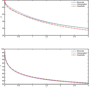
We first take a look at the critical stock prices below which the put option should be exercised
immediately. Figure 1 plots the critical priceS∗
τ as a function of time to maturityτ for two fixed parameter vectors (r, δ, σ). In both subplots, we set K = 100, and σ = 0.4. The top subplot is
for r = 0.04, and δ = 0.08, while the bottom subplot uses r = 0.08 and δ = 0.04. A very nice common feature of the quadratic approximation and the interpolation method is that they both
have the correct asymptotic critical stock price as τ →0+, which is given by
S∗
0+ = min(K, rK/δ). (59)
The choices of r and δ are made such that the theoretical asymptotic critical stock prices at
τ = 0+ are different for the two subplots. For the top subplot, the theoretical value is 50, while it is 100 for the bottom subplot. The general conclusion we can draw from this figure is that
at least for the particular parameters used in the figure, both the quadratic approximation and interpolation method produce relatively accurate critical prices.
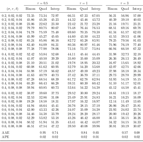
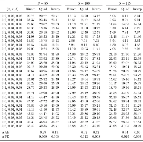
Table 1 presents a more thorough study by considering different parameter combinations of
r,δ,σ andτ. Three maturities are chosen, namely, 0.5, 1, and 3 years, representing short-term,
medium-term, and long-term options, respectively. The interest rates and dividend rates are set to be either 0.02, 0.04, or 0.08. Thus the ratio r/δ ranges from small (0.25) to fairly large (4.00). The volatilities are set to be either 0.2, 0.4 or 0.6 to represent low, medium and high
volatilities. For all the options, the strike priceKis fixed at 100. Results from three methods are presented: the Cox, Ross and Rubinstein’s binomial tree method with 10000 time steps (treated
as the true values), the quadratic approximation in Barone-Adesi and Whaley (1987), and the interpolation method in this paper. The average absolute error (AAE) and average percentage
error (APE) for the relative columns are also presented. The average percentage error is defined as the ratio of the absolute approximation error to the binomial tree value. A quick look tells us
6
that the two methods give very similar results on average. For all three maturities, the average percentage error is about 2% for both methods. The larger errors of the interpolation method
seem to concentrate in the parameter region whereδ is small.
One of the motivations of this paper, besides searching for an efficient and accurate analytical
approximation, is to take a more systematic look at the interpolation method first proposed in Johnson (1983) and extend it beyond the simple case of zero dividend rate. The quantity of a
lot of interest in this interpolation method is the weight α. In Johnson’s paper, α is fitted by regression using a limited number of American options from Parkinson (1977) and Rubinstein and Cox (1982). Our closed-form expression in equation (30) allows us to take a detailed look
at α without too much computational burden. In our approximation, the S dependence of α
is captured completely in the factor Sq(r−δ,r/Φ)
, and the constant A has no S dependence. By
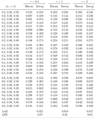
the value matching condition in equation (23), the constant A has an interpretation of being the weight of interpolation at the critical stock price. Table 2 presents the weight A in our
interpolation method as a function of volatility σ, interest rate r, and dividend rate δ for the same parameter combinations we used in Table 1. As the value matching condition is satisfied
in both the binomial tree model and the interpolation method, the differences inAin these two methods are purely due to the differences in the values for S∗
τ. As we see, the values ofA have a wide range as the parameters change. The smallest value ofA from the binomial tree model in the table is 0.087 while the largest is 0.686. The interpolation method gives fairly accurate estimates of A. The average absolute errors are about 0.2 for all three maturities, while the
average percentage errors are 7% or below.
By looking more carefully the numbers in Table 2, we see that at least for all the parameter
combinations presented in the table, A is an increasing function of σ if we keep r, δ and τ
constant. However, the dependence of A on r, δ, and τ are not as simple. In general, A is
an increasing function of r, but there are a couple of exceptions, for example, when σ = 0.2,
δ = 0.08 and τ = 0.5. Also, A is generally decreasing in δ, except for the first three rows.
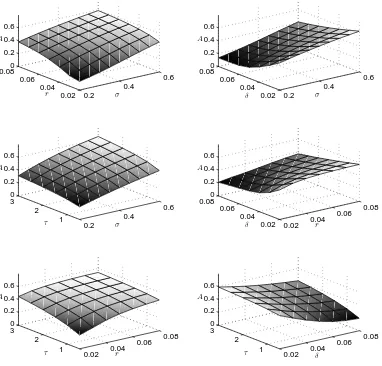
Finally, A is usually an increasing function of τ, the parameter combination σ = 0.2,r = 0.08 and δ = 0.02 being one exception. Figure 2 gives us a more continuous look at the dependence ofAon the parameters (σ, r, δ, τ). The subplots in the figure reinforce the rough observation we
made from Table 2 thatA generally increases withr,σ and τ, but decreases withδ. That A is increasing in r and decreasing inδ agrees with our intuition. Recall that A can be considered
a penalization for having to deliver the stock and receiving the cash at the same time. If r is much larger than δ, then the difference of costs between delivering the stock at some random
time and delivering it at maturity decreases. On the other hand, we are more likely to early exercise in order to receive the cash earlier. These two push the American option price closer
and τ is not intuitive to us. Thus, the numerical study of the interpolation parameter A adds our understanding on the interpolation method, initially studied in Johnson (1983).
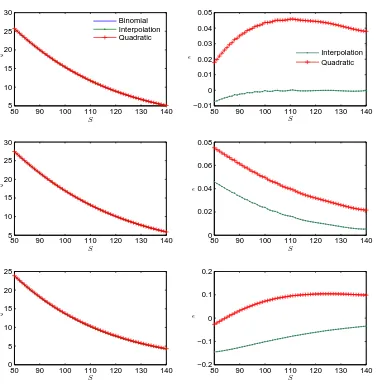
We are now ready to take a look at the pricing performance for the American put options. Figure 3 plots the American put option prices as a function of the current stock price S (left
subplots), as well as the approximation errors for the quadratic and interpolation methods (right subplots). In all the subplots, K = 100, σ = 0.4, and τ = 1. The pairs of interest rate r and
dividend rate δ used in the top, middle and bottom panels are (0.04,0.04), (0.04,0.08), and (0.08,0.04), respectively. As we see, both the quadratic and interpolation methods are quite accurate. All three pricing curves seem to be on top of each other in the three left subplots. The
right subplots give us a finer look at the pricing performance. The two methods give similar errors, with the interpolation method seems to be more accurate for out-of-the-money options.
This is to be expected, since for out-of-the-money options, the two bounds in the interpolation get closer to each other.
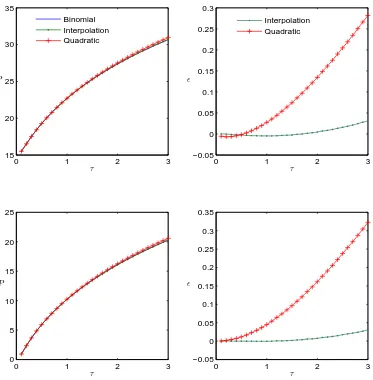
Figure 4 allows us to take a quick look at the performance of the methods along a different dimension, namely, the time to maturityτ. The left two subplots plot the option prices from the
three methods, while the right subplots plot the pricing errors of the interpolation and quadratic approximation methods. In all the subplots,K = 100, σ = 0.4, and r=δ = 0.04. The current
stock prices used in the top and bottom subplots are S = 85 and S = 115, respectively. These two approximately represent out-of-the-money and in-the-money options. As we see, both the quadratic and interpolation methods are still quite accurate for τ ranging from 0.5 to 3 years.
However, at least for these parameters, the interpolation method performs better for longer-maturity options than the quadratic approximation. This is consistent with the findings in Ju
and Zhong (1999) that the performance of the quadratic approximation deteriorates when τ
increases.
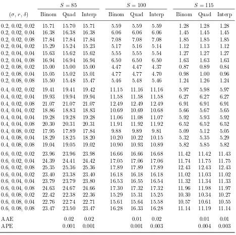
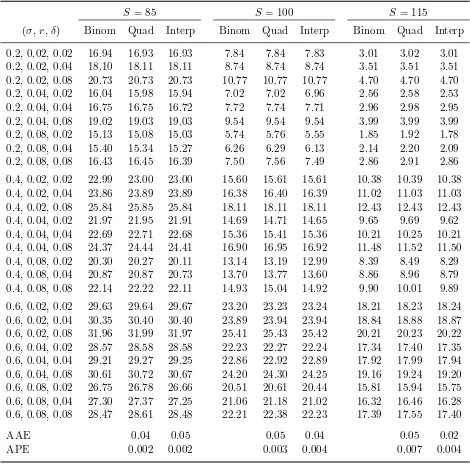
Tables 3, 4 and 5 take a more detailed look at the performance of the quadratic approximation and interpolation methods in pricing American put options by looking at short-term,
medium-term and long-medium-term options separately. More specifically, we fix the maturity τ in Tables 3, 4 and 5 to be 0.5, 1 and 3 years, respectively. The interest and dividend rates are set to be either 0.02, 0.04, or 0.08. The volatilities are set to be either 0.2, 0.4 or 0.6. The strike K is fixed
at 100. The current stock prices are chosen to be 85, 100, 115, representing roughly in-the-money, near-the-money and out-of-the-money put options. Table 3 shows that the performance of the
two methods is extremely similar for short-term options, with the average percentage error for both methods within 0.5%. Tables 4 and 5 show that the accuracy of both methods decreases
somewhat as the maturityτ increases, especially for the quadratic approximation. In all three tables, the relatively larger errors for the interpolation method are usually associated with small
In general, the interpolation method performs better than the quadratic approximation for long-term options and out-of-the-money options. Although not reported in the tables, we also
compute option prices for S = 130 and 145. For these stock prices, the interpolation method clearly outperforms the quadratic approximation.
B. American option pricing in Heston’s stochastic volatility model
We now take a look at the performance of our interpolation method for Heston’s stochastic volatility model. For simplicity, we use the zeroth-orderσv-expansion which amounts to replace
σwithσein equation (52). In the first part of our numerical study, we use the same parameters as in Ito and Toivanen (2006) and Medvedev and Scaillet (2009) in order to compare the accuracy.
That is, r = 0.1, δ = 0, κv = 5 or 2.5, θv = 0.16, σv = 0.9 or 0.45, ρ = 0.1. Time-to-maturity is 3 months (0.25), and strike price is set at 10. Two different instantaneous volatilities are
considered: vt= 0.0625 andvt= 0.25.
Before we look at the accuracy, it is worthwhile pointing out that our method takes about 0.02
seconds to price one option under the stochastic volatility model in MATLAB. The bulk of the computing time is spent computing the inverse Fourier transformations as each iteration would
require the computation of two European option prices. Since the approximation in Medvedev and Scaillet (2009) takes about 0.1 seconds to compute one option, it seems that our method is about 5 times faster (some caution has to be taken with this claim as the comparison might not
be fair due to possible different computer powers). Also, our method is not as “bulky”. The core algorithm of our method takes less than 20 lines of MATLAB code apart from the inverse
Fourier transformation for computing the European option prices.
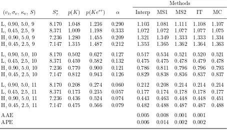
Table 6 reports the results for the performance of our interpolation method (coupled with
a zeroth-order σv-expansion using the time-averaged expected variance) together with other existing methods under Heston’s stochastic volatility model. The other models include: the
numerical method in Ito and Toivanen (2006), the two 5-th order approximations in Medvedev and Scaillet (2009), and Monte-Carlo method (taken from Medvedev and Scaillet (2009)) in
Longstaff and Schwartz (2000). These are abbreviated as Interp, IT, MS1, MS2, and MC, respectively. Also reported are the critical stock price, two European put option prices p(K) and p(Kerτ) used as lower and upper bounds, and the interpolation weightα (which is not the
interpolation parameter A). The average absolute error (AAE) and average percentage error (APE) are also presented assuming that the prices from MC are the true prices. As we see
from the table, our method is fairly accurate with an average percentage error of only 0.6%, and slightly more accurate than the approximation 1 in Medvedev and Scaillet (2009). It is also
change the result much. For example, using the instantaneous variance vt itself or the Black-Scholes implied volatilities forp(K) orp(Kerτ) in place ofσ results in average percentage errors
of 0.8%, 0.7% and 0.7%, respectively. The approximation 2 in Medvedev and Scaillet (2009) seems to be more accurate than our interpolation method. The same is true for Ito and Toivanen
(2006), although our method is faster than both of these two other methods. Also, one has to take caution that the parameters in this table are not very typical. For example, the magnitude
of ρ and τ are fairly small. Since Medvedev and Scaillet (2009) relies on a small-τ expansion while our method approaches the true perpetual American option price as maturity goes to infinity, it is possible that our method will have an advantage for long-maturity options. Also,
for computational efficiency, we have coupled the interpolation approximation with a zeroth-order σv-expansion which understates the option prices. The accuracy of the interpolation
method would be improved if we use numerical methods to compute the perpetual American option price and its partial derivative, although at the cost of lower computational efficiency.
The availability of an efficient and accurate quasi-analytical American option pricing algo-rithm under stochastic volatility model allows us to take a detailed look at the dependence of
various quantities such as S∗
τ,A, and C(S, τ, K) on parameters of interest such asvt,σv,κv,ρ,
θv, etc. This has considerable value as a detailed understanding of these dependence properties
is still lacking in the literature.
Figure 5 plots the critical stock prices for American put options under Heston’s stochastic volatility model as a function of the instantaneous variance vt, the volatility of varianceσv, the
mean-reverting strength κv, and the long-run mean instantaneous variance θv. Three different values of shock correlation ρ are plotted on each of the four subplots: −0.6 (the curves marked with∗), 0 (the curves with no markers), and 0.6 (the curves marked with +). The base parameter values are: K = 10, r = 0.1, δ = 0, vt = 0.25, σv = 0.7,κv = 3, andθv = 0.10. The subplots
have no dependence on the current stock price S since the critical stock price is not a function of the current stock price. On each of the four subplots, one parameter (thex-axis) is relaxed
to vary in a fixed region as shown in the subplots. For example, the instantaneous variance is allowed to vary from 0.01 to 0.49 (corresponding to instantaneous volatility going from 10% to 70%). Notice that the regions are chosen to be quite wide in order to have a complete view.
As we see in the figure, regardless of the sign of the correlation coefficient ρ, the critical stock price S∗
τ is always decreasing in the instantaneous variance vt and the long-run mean θv. In particular, S∗
τ is quite sensitive in vt. This agrees with our intuition that when the volatility gets higher, holders of American put options become more reluctant to exercise the option and
the stock price has to drop much lower in order to induce him to exercise the option early. Consistent with established results such as those in Lewis (2000), when ρ = 0, the volatility
when ρ is large in magnitude, Sτ is increasing in both σv and κv if ρ < 0, and decreasing in both σv and κv if ρ > 0. This runs somewhat against our intuition that the effect of σv and
κv should be opposite to each other, as one parameter tends to amplify the effect of stochastic volatility while the other tends to diminish it. Nonetheless in extensive numerical analysis we
find that S∗
τ behaves similarly as σv and κv change is a very robust property. For example, changing the relative magnitude ofθv and vtdoes not affect this property at all. Finally, in all
four subplots, the critical stock price S∗
τ is smaller when ρ > 0 than when ρ < 0. This agrees with our intuition. The reasoning goes as follows. Suppose ρ >0. Then when the stock price
S drops, the option tends to be more valuable. However, because of the positive correlation,
there is a larger possibility that the instantaneous variance vt would also drop, which reduces the option option. The situation is different when ρ < 0, where the effect of a drop in S is
reinforced by an increase in vt. This is the origin of the volatility skew in Heston’s stochastic volatility model. Therefore, whenρ <0, an American put option holder would tend to exercise
more than ifρ >0, resulting in a largerS∗
τ forρ <0.
Figure 6 plots the interpolation parameter A for American put options under Heston’s
stochastic volatility model as a function of the instantaneous variance vt, the volatility of vari-anceσv, the mean-reverting strengthκv, and the long-run mean instantaneous varianceθv. The
parameter values are the same as those in Figure 5. Recall that A is the interpolation weight
α if S = S∗
τ and is not a function of the current stock price S. As we see, the interpolation parameter A is not very sensitive to all the parameters, especially when ρ = 0. This probably
can explain partially why our interpolation method is so accurate given its simplicity. Again, the interpolation parameter is larger when ρ < 0 than when ρ > 0 on all four subplots. The
interpolation parameter A is always increasing in vt in order to produce higher early exercise premium when volatility gets larger. The dependence of A on θv is not very strong. Also, if
ρ <0, Ais increasing inσv andκv. The situation is opposite whenρ >0.
Figures 7 and 8 further plot the interpolation parameterA for American put options under
Heston’s stochastic volatility model as a function of the instantaneous variancevt, the volatility of variance σv, the mean-reverting strength κv, and the long-run mean instantaneous variance
θv. The difference is that in Figure 7 we setS= 9 so that the options are “in-the-money”, while
in Figure 8 we set S = 11 so that the options are “out-of-the-money”. Comparing these two graphs, we see that the effect ofρis completely opposite for in-the-money and out-of-the-money
options. A negative ρ tends to increase the price of an out-of-the-money American put option while decrease the price of an in-the-money put option, a result well-known for the European put
option case. See the original paper of Heston (1993) or page 70 of Lewis (2000). The American put option price on both graphs is increasing in vt and and θv, which agrees well with our