Informed trading in parallel bond markets

BIROn - Birkbeck Institutional Research Online

Paiardini, Paola (2009) Informed trading in parallel bond markets. Working

Paper. Birkbeck College, University of London, London, UK.

Downloaded from:

Usage Guidelines:

Please refer to usage guidelines at or alternatively

ISSN 1745-8587

Birkbeck Workin

g

Pa

p

ers in Economics & Finance

School of Economics, Mathematics and Statistics

BWPEF 0908

Informed Trading in Parallel Bond

Markets

Paola Paiardini

Birkbeck, University of London

Informed Trading in Parallel Bond Markets

Paola Paiardini†

Abstract

In this paper we investigate the presence of asymmetric information

in the parallel trading of ten-year government fixed rate bonds (BTP)

on two secondary electronic platforms: the business-to-business (B2B)

MTS platform and the business-to-customer (B2C) BondVision one.

The two platforms are typified by a different degree of transparency.

We investigate whether the probability to encounter an informed trader

on the less transparent market is higher than the corresponding

prob-ability on the more transparent one.

Our results show that on BondVision, that is the less transparent

plat-form, the probability of encountering an informed trader is higher.

Finally we perform a series of tests to check the robustness of our

estimates. Two tests do not meet the hypothesis of independence.

Nevertheless, these findings do not controvert the hypothesis of our

model, but call for further analysis.

JEL codes: C51; G10; G14

Keywords: Market microstructure; Informed trading; Parallel

trad-ing; Transparency

∗

I am grateful to Stephen Wright, Emanuela Sciubba, Ron Smith, Sergio Ginebri, Luca Arciero, Raffaele Lombardi, Stefano Falciani and to all participants to Jamboree Seminar and to41stMoney Macro and Finance Conference for useful comments.

†

1

Introduction

Nowadays the scenario for the investors has notably changed with respect to

a non so far past. The quick progresses in Information and Communication

Technology have outstandingly changed the organization of securities

trad-ing in Europe and worldwide. Tradtrad-ing no longer takes place in a physical

location, while trading floors and telephone networks are more and more

moving over for transactions conducted via electronic trading platforms.

Today investors have the possibility to select among a great variety of

choices what is the best suitable for their own requirements and execute their

trades. Financial securities are not only traded on regulated markets but also

on new electronic trade platforms, which are characterised by different levels

of intermediation. There has been a notable raise in the development of

these new electronic markets, where are traded securities that were already

traded in non-electronic existing markets.

All these changes have driven a great increase in theoretical works

con-cerning the analysis of market microstructure, furthermore the recent

avail-ability, at relative low costs, of high frequency datasets have contributed to

a notable increase also in empirical works.

The coexistence of multiple markets for the same asset is a pervasive

phenomenon; financial securities may trade simultaneously on a number of

markets, so the main issue of a trader is to decide how to allocate his

or-ders across the different trading venues. As a consequence, all these

trad-ing venues compete for order flow, so it is really important to understand

how inter-market competition affects market quality. This scenario raises

questions about the coexistence of markets that differ along a variety of

There exists an extensive market microstructure literature on single

mar-kets, which analyses their characteristics, how they work and so on, however

there is a scarce literature on intermarket competition, where traders can

trade a same asset simultaneously on several markets and on the

interac-tions among different market segments. Government bond market has been

traditionally divided in an inter-dealer and a dealer-to-customer segment,

however, economic researches, which had analysed these two dimensions,

had focused their attention only on the more liquid inter-dealer segment

ignoring the dealer-to-customer segment.

There is a narrow theoretical and empirical literature which had

nib-bled at the impact that the existence of electronic trading platform have on

traditional markets and the chances of survival of both. One of the most

promising approach which is catching on the literature about market

mi-crostructure and more precisely, concerning how parallel trading of a security

on several markets can influence prices, is the sequential trade model. This

model combines both econometric analysis and economic theory, which was

initially used simply to analyse information aspects of the price discovery

process on financial markets.

In a sequential trade model there are three economic agents who are in

a dynamic interaction: a market maker who supplies liquidity to the market

by continuously posting prices at which the security may be bought and

sold, and two types of traders, who differ with respect to their information

set on future price movements. In this framework the market maker sets

prices without knowing whether any trader has superior information about

the fundamental value of the security. The main aim of these models is to

analyse the effects of asymmetric information among market participants on

In this work we construct a sequential trade model to consider parallel

trading on two platforms of the secondary bond markets, MTS (Mercato

Telematico dei Titoli di Stato) and BondVsion, which are typified by a

dif-ferent degree of transparency. The Italian government bond market is one

of the largest in the world. We investigate whether the probability to

en-counter an informed trader on the less transparent market is higher than the

corresponding probability on the more transparent one.

The paper proceeds as follows. Section 2 briefly reviews sequential trade

models under asymmetric information for equity and bond markets. Section

3 analyses the institutional environment. Section 4 describes the asymmetric

information model used to analyse the parallel trading on the two platforms.

Section 5 illustrates the database. Section 6 contains the empirical analysis.

Section 7 concludes.

2

Models under asymmetric information

There are two different approaches to model sequential securities market

behaviour in the presence of asymmetric information. One approach is

Wal-rasian batch models and another is sequential trade models.

In the Walrasian approach, market makers observe the net order from

traders and set a single price, at which all orders are being executed. The

trading process is a sequence of auctions based on requests to buy or sell

a specified number of securities at the market price. These models do not

allow to characterize the bid-ask spread, but focus on the effects of order

placement by informed and uniformed traders on prices. The pivotal work

in this approach is that of Kyle (1985).

The three classical papers that mathematically formalised sequential

(1985) and Easley and O’Hara (1987).

Copeland and Galai (1983) construct a one period model, where market

makers pricing, given that some fraction of traders have superior information

on the assets true value. The market maker is risk neutral and sets quotes

to maximize his expected profit. Uninformed traders know how the general

pricing process works, but they do not know the true value of the asset. The

market maker cannot identify informed traders, however he knows the

prob-ability that any trade comes from an informed or from an uninformed trader.

Therefore, the quotes set by the market maker emerge from a profit

maxi-mization problem, because he calculates the expected profit from any trade,

taking into account the probabilities of losing to the informed and gaining

to uninformed. The weakness of this model is that all private information

is made public after a trade is conducted. Even when repeated rounds of

trading are allowed, the expected loss of the market maker will remain the

same, so he has no incentive to change his quotes. This means, that in this

framework, the trading process is not informative at all. However, if private

information is revealed after each round, sequences of buys and sells may

reveal the underlying information process and affect the behaviour of prices.

The learning process from the order flow has been analysed in a dynamic

framework by Glosten and Milgrom (1985) and Easley and O’Hara (1987).

Informed traders will reveal their information by selling the asset, if they

know bad news and buying it if they observe good news.Therefore, the fact

that someone wants to sell may be interpreted as a signal to the market

maker that bad news have been received by this trader, but it may also

mean, that the trader is uninformed and simply need liquidity.

Easley and O’Hara (1987) introduced the notion of information

does not observe the information event, he knows that there are traders who

always know either good or bad news. In this work, instead, it is introduced

a third possibility, i.e. the absence of any private information. In this case

the market maker will receive orders only from uninformed traders.

Another difference with the two previous works, is that the assumption

that a fixed number of securities is traded is relaxed. Now the market maker

can learn both from the direction and the size of trades. In Easley and

O’Hara (1987) may be traded two different trade sizes,large andsmall

quan-tities. It is assumed that uninformed traders will transact both quantities,

otherwise trade size will identify the type of trader unambiguously.

Both types of models have their deficiencies and their merits. However,

the sequential trade model is more corresponding to the actual features of

the government bond markets and, in particular, to the data available for

the empirical analysis. All these aspects make us prefer a sequential trade

approach to a batch approach. It represents not only a theoretical model of

the effects of information asymmetries on price setting behaviour, but it also

provides a coherent framework that can be used to estimate structural

pa-rameters of the model form observable quantities that are typically contained

in high frequency transactions data sets from financial markets.

2.1 Sequential trade models under asymmetric information

In this section we will briefly review some of the sequential trade models

that have been used to analyse securities behaviour under asymmetric

infor-mation. We will use the model used in Easley et al. (1996b) as the basic

sequential trade model, since it may be considered a simplified version of

its predecessors Easley and O’Hara (1987) and Easley and O’Hara (1992).

basic framework for more complex models.

Easley et al. (1996b) setup a mixed discrete and continuous time

se-quential trade model of the trading process. In this framework traders arise

because of the interactions of three types of economic agents: informed and

uninformed traders and a risk-neutral, competitive market-maker. The

ar-rival rates of informed and uninformed traders are governed by independent

Poisson process and the likelihood of the occurrence of three different types

of information events (no news, good news and bad news) which are chosen

by nature every day, before the first trade take place. In this model, the

difference between bid and ask quotes arises only because of asymmetric

in-formation of market participants about the occurrence of inin-formation events.

Other components of the spread, such as those caused by maintaining large

inventory imbalance, or by the exercise of market power by a monopolist

market maker are left aside.

Other models, add to the basic sequential trade model in Easley et al.

(1996b) trade size and time effects. Theoretical foundations for the inclusion

of these aspects have been developed in Easley and O’Hara (1987) and Easley

and O’Hara (1992). In these works the trading day is divided into discrete

time intervals, where each interval is long enough to accommodate just one

trade. This assumption allows to define a third event, no-trade event, in

addition to buys and sells.

In Easley et al. (1996b) no-trade intervals may arise in the course of the

trading day but they are treated implicitly as zero observations of the buy

and sell sequences. Throughout the introduction of the no-trade events, the

duration between trades will have an effect on the market maker pricing

behaviour, because long durations between trades indicate the absence of

lower the spread, when the intensity of trading is low. In this catheogory

lies the works of Easley et al. (1997a), Easley et al. (1997b).

Easley et al. (1997a) additionally distinguish between two different trade

sizes, small and large trades. Easley et al. (1997b) introduce also the

possi-bility that uninformed traders condition their trades on the observed order

flow, thus inducing serial correlation in the observed trading process. They

argue that uninformed traders will consider the trading history when placing

their orders.

Finally, a further extension of the basic sequential trade model is to take

in consideration parallel trading of a same asset in two different market

de-signs. In this framework lies the works of Easley et al. (1996a), Easley et al.

(1998) and Grammig et al. (2001). The first work analyses the possibility

that the practice of cream-skimming arises in trading in two regional

mar-kets1.

Easley et al. (1998) derive a model for parallel trading in stock and option

markets. They investigate whether derivatives markets are used only for

risk hedging purposes, or whether they also constitute a venue for informed

traders.

Grammig et al. (2001) construct a sequential trade model, that allows

for parallel trading on a floor trading system requiring physical presence

of all traders and a screen trading system, that enables traders to remain

anonymous.

Following Kokot (2004), a summary of frameworks and principal results

of all the above models is reported in Table 1.

1_{Cream-skimming is the practice on the base of which, restricting the types of orders}

2.2 Models which analyse the bond market

In spite of the importance of this market, there are not many models who

analyse the bond market. Dunne et al. (2007) consider the interaction

be-tween the inter-dealer (B2B) and the dealer-to-customer (B2C) segments of

the European bond market. They develop a model to understand the quote

dynamics in both segments and their interrelationship. They theorize that

dealers are willing to hold short or long inventory positions within defined

limits. Dealers are rewarded for this by arbitrage opportunities between

the B2C and the B2B spreads. Dunne et al. (2007) find that a large share

of the retail quotes and an even larger share of retail transactions occur

within the B2B spread. Their model explain the relatively high inter-dealer

spreads with the higher adverse selection risk carried by quote submission

in the inter-dealer market. However, this model has some weakness. Firstly,

the theoretical framework implies a rich set of predictions about the quote

dynamics, but testing these predictions requires dealer specific inventory

in-formation, which is not available. Secondly, this model lies on the inventory

cost, but one of the characteristics of the bond market is the possibility of

hedging, that is in contrast with this assumption.

He et al. (2006) analyse the US government bond market. They use

a sequential trade model to compute the probability of information-based

trading . However, this model does not completely correspond to the market

design of sequential trade models, since they refer to a decentralized market

where each participant can post his own quotes and observe only a fraction

of the buys and sells.

Finally, Arciero (2006) uses a sequential trade model to analyse an

elec-tronic centralized market where only market makers can post bid-ask quotes

the inter-dealer segment of the bond market.

3

Institutional environment

For this research we take into consideration two electronic secondary bond

market platforms. One is MTS, acronym of Mercato Telematico dei Titoli di

Stato, that is a wholesale screen-based inter-dealer market for government

securities. As an inter-dealer platform, individual customers are not

admit-ted, instead only dealers are allowed to participate (i.e. banks and financial

institutions and other professional intermediaries who buy and sell securities

for their own account and on behalf of their customers).

The other one is BondVision, part of the MTS Group, it is a wholesale

screen-based multi-dealer-to-customer electronic market for fixed income

se-curities2. On BondVision, primary dealers trade directly with institutional

investors (insurance and asset management companies) by means of a

mul-tiple price auction system.

3.1 MTS

The original MTS market was first introduced in Italy in 1988, it was the

first electronic market created in order to enhance trading in the secondary

market of Italian government bonds. MTS has been the object of many

changes during the past years, starting with the diversification of securities

traded that now include, apart from the government bonds, also other fixed

income securities, that already had a market, also with considerable

pro-portions, but as an over-the-counter one. During the last two decades, the

MTS platform has been typified by many changes, the most important in

chronological orders were: the reform in 1994, the privatization into MTS

S.p.A. which took place in 1997 and the full anonymity of traders in 2003.

Table 2 gives a clearer picture of the changes which have taken place during

the last twenty years.

Table 2:

Changes in the Italian secondary bond market over the last two decades. Year Changes in market microstructure

1988 Setting up of MTS Italy

Start of regular re-openings of Treasury auctions Floor to bid prices abolished for T-bills; uniform price auction introduced for other bonds

1994 Treasury starts publishing timetable of auctions Electronic bid submission at auctions

Reserved re-openings for “specialists” in government securities

Continuous trading on the electronic retail market 1997 Monitoring functions to the MTS management board

Introduction of (ex-ante) anonymity of trades in the continuous trading market

Floor to bid prices abolished fr T-bills; uniform price auction introduced for other bonds

1998 First ad-hoc re-openings of Treasury auctions 1999 Setting up of EuroMTS

2003 Introduction of full anonymity of trades with the cen-tral counterpart (CCP) system

Source: Scalia and Vacca (1999) and Girardi and Piga (2007).

According to the MTS website, MTS S.p.A. is a regulated market,it

pro-vides wholesale electronic trading of Italian government bonds and other

types of fixed income securities. It is regulated by the Italian Ministry of

Economy and Finance, Bank of Italy and CONSOB. The majority stake is

held by Borsa Italiana (60.37 per cent), instead the remaining shares are

owned by international financial institutions3.

In 1999, with the introduction of Euro as the single European currency,

3

EuroMTS was created. It is a private London-based company that manages

the pan-European electronic trading platform for government and

quasi-government bonds denominated in Euro with at least5 billion outstanding.

Today EuroMTS is completely owned by MTS S.p.A.

In May 2001 was launched the EuroCredit MTS, a division of EuroMTS,

which operates as an electronic trading platform for high-quality covered

bonds. There are MTS Domestic Markets which list the government bonds

of the respective European country4.

The latest addition to the “MTS world” is the NewEuroMTS which is a

market built for the trading of euro-denominate government securities of the

ten new States entered in the European Union on 1 May 20045.

The Italian MTS is divided into two sections: one for spot trading where

bonds are exchanged for cash (MTS Cash) and the other is a market for

repurchased agreements (MTS Repos), in which who sells or buys commits

himself respectively to buy or sell the same security back at a future date

for a specified price6.

On MTS Cash segment there are two types of market participants.

Par-ticipants are qualified as dealers and primary dealers. Primary dealers act as

market makers, continuously quoting two-way proposals (bid and ask prices)

that are valid for all participants and for the whole day, unless they are not

modified, cancelled, automatically matched or hit by incoming orders.

Mar-ket takers have not any marMar-ket making obligation, they must simply accept

or not the quotes of market makers. Since primary dealers, unlike dealers,

4_{MTS has been successfully launched also outside the Euro area, e.g. MTS Japan Ltd.}

and MTS Israel in 2006.

5_{Countries whose bonds are eligible for trading in the NewEuroMTS Market include:}

Bulgaria, Cyprus, Czech Republic, Estonia, Hungary, Latvia, Lithuania, Malta, Poland, Romania, Slovakia, and Slovenia. www.mtsspa.it/index.php.

6

may also formulate proposals on any other tradable product and issue orders

for proposals made by other market participants, they can act both as price

makers and price takers7.

Within the group of primary dealers, for purposes of public debt

man-agement, the Ministry of the Economy and Finance selects a restricted list

of so-called Specialists who have to satisfy more stringent requirements. A

number of different short-term and long-term government bonds are traded

on the Italian MTS platform: floating rate treasury certificate (CCTs), fixed

rate bonds (BTPs), inflation-linked bonds (BTPis) and zero-coupon

securi-ties (BOTs and CTZs). There are precise rules governing the functioning of

MTS. There are some market making obligations, involving quoting a

min-imum quantity of a certain bond8, within a maximum spread (which varies

according to the maturity of the asset; it is higher for assets with a longer

maturity) for a minimum cumulative amount of time of at least five hours

per day. Finally when they post quotes they must also specify if it is ablock

or a drip quantity. The former represents the overall size of the proposal,

the latter the part of the order that is made visible to the market. The MTS

system actually works as a limit order book, any bond is assigned to many

primary dealers. The trading platform provides a lot of real-time

screen-based information to all market participants, who can easily know the state

of the market and observe the order flow.

The “live” market pages are:

1. Thequote page which gives the market makers the possibility to insert

offers; posted proposals can be modified, suspended or reactivated.

7

While this work is being carried out there are 29 primary dealers and 71 dealers, operating on the Cash segment.

8

2. Themarket depth page allows participants to see the best 5 bid and ask

prices for each security chosen together with its aggregated quantity.

3. Thebest page shows the best bid-ask spreads together with its

aggre-gate quantity for all products.

4. Thesuper best page shows the best price for bonds listed on both the

domestic MTS and the EuroMTS. Market maker who has access to

both markets can choose parallel quotation, i.e. they can

simultane-ously post proposals on both platforms.

5. Thelive market page shows for every bond the average weighted price

and the cumulative amount being traded so far.

Other rules concern trading time. The MTS market is divided into four

phases: pre-market time (from 7:30 am to 8:00 am CET), during this stage

only market makers are fully operative, they can issue and change their

proposals, but primary dealers can see only their own proposals.

The preliminary market time (from 8:00 to 8:15 am CET) during which

both primary dealers and dealers are active. However, during this phase, it

is not allowed the automatic matching among proposals. This is a useful

period because market makers have the opportunity to adjust their proposal

on the base of the other’s market makers observed prices.

Theopen market time (from 8:15 am to 5: 30 pm CET) during which it

is possible to send proposals and trade and also the automatic matching is

made available.

Finally the close market time during which no trading is allowed but

only the settlement of the contracts already concluded.

Anonymity prevents dealers form managing the counterpart risk,

service. Since the end of 2002 a central counterpart service has been active

on an optional basis, supplied by Cassa di Compensazione e Garanzia of

Italy and LCH. Clearnet of France. The role of the central counterpart is

to interpose itself between the parties involved in the trades, becoming the

buyer to the seller and the seller to the buyer in order to guarantee the

exe-cution of the trades by relying on the margin that the trades must deposit.

Thus, anonymity is guaranteed at least until the execution of trades, when

the identity of the parties could be revealed unless there is the use of the

central counterpart, in which case, anonymity is guaranteed also after the

execution of trades.

3.2 BondVision

BondVision is a multi-dealer-to-customer electronic bond trading market.

It is another regulated market, supervised by the Italian Ministry of

Econ-omy and Finance for the government bonds and by CONSOB for the

non-government trading section. It was launched in 2001 in response to

contin-uous requests from institutional investors for access to the liquidity of the

MTS markets.

BondVision allows participants, qualified as primary dealers, to trade

directly with clients, qualified as institutional investors, such as investment

managers, hedge funds, private banks (for this reason we classify BondVision

as another wholesale market, according to the definition on the Bank of Italy,

rather than as a retail market, as defined in some papers9.

On MTS, primary dealers insert a proposal on the Best Page and all

the market participants hit the bid or ask price depending on whether they

want to sell or buy. Subsequently the contract is finalised, i.e. the "‘click and

9

trade" system, and finally settlement instructions are automatically

gener-ated.

On BondVision platform, instead, a contract is generated only as a

con-sequence of a request from a client (end-user). Three phases characterize the

process on BondVision platform: request, proposal and acceptance.

During the request phase, clients can select a product, the direction of

their trade (if they want buy or sell) and the amount of their title and via

the Request for Quote (RFQ) or request for switch quote (RFSWQ)

func-tionalities, simultaneously send an electronic trade request to a maximum

number of dealers, hence starting an auction10.

During the proposal phase, each dealer participating in the auction send

a responding bid or offer allowing the client to execute the trade at the

best price. Dealers are not required to provide quotes when requested and

clients are not obliged to accept any of the quotes they receive. They have

90 seconds to decide. Also on BondVision there is a Best Page, however the

prices are indicative and not executable and it is absolutely not necessary

that the requests are present in a list on the Best Page, so there is not

a proper order book as for MTS. Furthermore, on BondVision, the client

can also ask for a different settlement time. On BondVision there exists a

minimum request obligation, the minimum lot is 100.00011. We have to

point it out that BondVision is not an anonymous environment, since, when

a client send a RFQ, he selects the dealers and the dealers selected, in turn,

know who is the client who sent them the request. Furthermore, when a

10_{Each client is not allowed to send a RFQ to every dealer, but he can request quotes}

only to a certain number of dealers (At the moment five). More precisely, when a new client joins BondVision, he gives preference to some dealers and each dealer selected, in turn, agrees to trade with the client and chooses the titles on which is willing to offer liquidity.

11

dealer sends a proposal to answer a request of a client, he knows the prices

that other dealers involved have quoted but he does not know their identities.

During the last phase, the contracts concluded are regulated directly by

the parts. There is any regulation for the settlement. Thus, since there is

any regulation for the settlement procedure, of course there is no possibility

to make use of the central counterpart, so there is not anonymity neither in

this phase.

4

The model

4.1 The information and trading structure

Our model belongs to the class of “sequential trade models” that date back

to the work of Glosten and Milgrom (1985). More precisely it lies in the

category of those works which use a modelá la Easley and O’Hara (1992).

These types of models introduce as a difference to the classic sequential trade

model an additional source of uncertainty, that they define event uncertainty

which arises because an information event could have occurred or not.

We modify this reference model with adjustments that partly reflect those

made by other works and partly are changes introduced for our specific duty.

We consider an asset which has been contemporaneously traded on both

an inter-dealer and a dealer-to-customer platform, which are differing in

many respects. The true value of the asset is represented by a random

variableV. On the inter-dealer platform there are many market makers who

act competitively and continuously post bid and ask prices at which a trade

can take place.

Following the hypothesis of Glosten and Milgrom (1985) model, market

their model there is the presence of a single market maker (in our case there

are many market makers, but since they are assumed to act competitively,

the hypothesis can be considered still valid).

The rationality hypothesis implies that the market maker knows that the

order flow (i.e. the sequence of buys and sells occurred throughout the day)

is correlated with the true value of the asset, so he uses the indirect evidence

from the order flow to infer what this underlying value could be. The market

maker can learn from the order flow. Each time that he observes a buy, he can

infer that this trade comes either from an informed trader, who has positive

private information concerning the traded asset, or from an uninformed one.

On the contrary, if he observes a sell he can assume that the order comes

from an informed trader who knows bad news, or from an uninformed one.

The key to extract information from the order flow is a Bayesian

learn-ing process, throughout which the market maker reviews his beliefs about

the bid-ask quotes observing the sequences of buys and sells. Competition

dictates that any rent earned on trades would be put away by a competing

specialist. The market maker sets the bid-ask spread in order to have zero

expected profit and avoid entries. Competition drives profit to zero.

The risk neutrality assumption avoids that inventory matters, as it would

instead be the case with risk aversion or if the order flow were not observable

to all market makers. In this case, the market maker’s prices might reflect

information known only to himself, but with risk-neutrality such

inventory-based pricing effects will not arise.

The dealer-to-customer platform, is instead a quote-driven market where

clients send requests for quotes to dealers who are mainly those who act

as market makers on the inter-dealer platform. Thus, it is clear that the

concerned with our purpose is the dissimilar degree of transparency which

characterizes them, given that we are interested in investigating the presence

of asymmetric information in the treasury bond markets and empirically

in-specting if informed traders prefer the less transparent one. The trading

period is a trading day, trading days are indexed by i∈ [1, I]. Each

trad-ing day is divided into tradtrad-ing intervals of a given length, time within the

trading day is discrete and it is indexed by t ∈ [0, T] and at each interval

a trader is selected. The length of the trading interval is chosen to make

possible at least one trade in each interval. The choice of a trading day

as trading period is certainly arbitrary and not so respondent to reality,

be-cause prices could adjust to new information in minutes and new information

events could happen more frequently than once per day. However, since the

trading period is defined as the average time it takes to incorporate private

information into prices, the choice of the trading day as trading period seems

plausible. Moreover, Easley and O’Hara (1992) uphold the choice of a

trad-ing day as tradtrad-ing period because, ustrad-ing their words,“[. . . ]what matters for

our analysis is the learning confronting market participants. This is most

easily characterised by adopting the fiction of a trading day and assuming

that information events occur only between trading days”12.

Each trading day, before trading begins, nature selects whether or not

an information event will occur. Information events are assumed to be

inde-pendently distributed13.

If an information event has occurred, this means that there has been the

delivery of a signal (Ψ) about the true value (V) of the asset; this happens

with probability α. When an information event has occurred, the type of

12_{Easley and O’Hara (1992), p. 580.} 13

signal can be a high signal (H) in case of good news (g), with probabilityδ,

or a low signal (L) in case of bad news (b), with probability(1−δ).

On the contrary, when no private information is disclosed, we will have

a no-event day, in which case the signal isΨ = 0, with probability(1−α).

If there is no event, the probability of a trade is given respectively byQ and

O for the quote-driven and the order-driven platforms and, similarly, that

of a no trade by (1−Q) and (1−O) always for the two platforms.

Let (Vi)Ii=1 be the random variable giving the value of the asset at the

end of each trading day. During day i, if an information event occurs, the

value of the asset conditional on good news is Vi = E[V|Ψ = H], on bad

news isV_i =E[V|Ψ =L].

The value of the asset if no news occurs isV_i∗ =δV_i+ (1−δ)Vi, (assuming,

of course, V_i< V_i∗ < Vi).

What we have been describing so far represents what Easley et al. (1997a,b)

called theinformation process which describes the information state that is

reached only at the beginning of each trading day. Here after, there is the

beginning of what could be defined as thechoosing process, which illustrates

the choice of the platform from the market maker, which is not

necessar-ily a mutually exclusive choice, since the market maker can take a different

position contemporaneously on both platforms.

In our model market makers decide on which platform to trade, they

choose to trade on the inter-dealer quote-driven platform with probabilityβ

and on the dealer-to-customer order-driven platform with probability(1−β).

The last stage is, using again the words of Easley et al. (1997a,b), the

trading process which describes the traders’ choices and their behaviour

dur-ing each information state. For the trade in the next traddur-ing interval, only

day.

At each trading interval a trader is selected. If an information event has

occurred, an informed trader is selected with probability µQ on the

quote-driven platform andµOon the order-driven platform and then he can choose

whether to buy or sell with respective probabilities.

Informed traders know, before the trading day begins, whether the true

value of the asset will take a high or low value.

At each trading interval an informed trader will buy the asset if nature

has delivered good news, with probability one, and he will sell it, with

prob-ability one, if the nature has delivered bad news.

Similarly, an uninformed trader is selected with probability (1−µQ)

(quote-driven platform) and(1−µO)(order-driven platform), and again he

decides to buy, sell or not to trade with the respective probabilities.

If no information event has occurred, all traders are uninformed and the

trader selected may choose again to sell, buy or not to trade. Thus, an

informed trader will always trade provided that the ask price is below the

value of the asset in case of a high signal or the bid price is above the value

of the asset in case of a low signal.

An uninformed trader, instead, will trade only on the base of his portfolio

purposes.

The market maker knows that there are informed and uninformed traders

in the market, but he does not know with which type of trader is actually

trading. Furthermore, we assume that the arrival rates of uninformed and

informed traders in both markets is given, however, there is no reason to

think that these arrival rates must be equal between the two markets.

The addition to the market structure of the event uncertainty at the

(1985) model, implies that in some time intervals there could be no trade.

In this perspective, market makers learn not only from trades but also from

the lack of trades because each event provides an information.

Since informed traders are assumed always to trade if selected, all the no

trading intervals happen because an uninformed trader was selected and he

has decided not to trade.

Given these assumptions, we might expect that the probability of a no

trading interval occurring is negatively correlated with the probability of

a newsworthy event, Brown et al. (1999) reach the same conclusions, using

only order data, so they consider, instead of no trading intervals the no order

intervals.

However, we have to bear in mind that a no-trade observation is not a

sufficient component by itself to infer whether there has been an information

event. In fact, this can occur both when there has not been any information

event and when a trader decides not to trade for portfolio reasons. At the

same time, we have to notice that a no-trade outcome is more likely to

occur when there is no new information; this statement can be confirmed

simply looking at the probabilities. Consider, as an example, only the

quote-driven market. If there is no new information event, the probability of no

trade is given by (1−Q), instead if an information event has occurred

and the uninformed trader has decided to not trade, this probability falls

to (1−µQ)(1−Q), because now there are both informed and uninformed

traders in the market.

For our model, we are considering the parallel trading of a same asset

on two trading platforms of the secondary government bond market. In

constructing our model we extend the model of Easley and O’Hara (1992)

trading in the German stock market, where an anonymous electronic market

and a non-anonymous trading system coexist.

In the afore mentioned work, the authors wonder about the coexistence

of markets with differing degrees of anonymity and wondered which traders

prefer which market. They test empirically the hypothesis that informed

traders prefer the anonymous market.

In our specif case, we want to investigate the presence of informed and

uninformed traders on both platforms and we want to verify the assumption

that the presence of informed traders is grater on the market characterised

by a higher degree of transparency. On both markets there is the presence of

informed and uninformed traders. Informed traders buy on the two platforms

with probability one if they know good knows and zero if they know bad

news; uninformed traders instead, after having decided to trade, can choose

if buy with a probability η or sell with probability (1−η). The overall

The evolution of prices through the day follows a Bayesian learning

pro-cess14. The market maker does not know neither if an information event has

occurred nor if it is a good or a bad event. However, the market maker can

observe all trading activity, this allows him to capture information and to

revise his beliefs. This revision, in turn, causes quotes and prices to adjust.

Consider the market maker acting on the inter-dealers quote-driven

plat-form15. At the beginning, when market opens, the market maker beliefs

about the unconditional probabilities for no news (n), good news (g) and

bad news (b) are given by: PQ(0) = (1−α, αδ, α(1−δ). After each trade

interval, these probabilities are updated, using Bayes’ rule.

PQ(t) = (PQ,n(t), PQ,g(t), PQ,b(t)) is the vector of the subjective

probabili-ties conditional on the trade history in the market prior to time t.

The expected asset value, conditional of the trade history is:

EQ(Vi|t) =PQ,n(t)·Vi∗+PQ,g(t)·Vi+PQ,b(t)·Vi (1)

The trade outcome at timet is given by:

θt∈ {N T, SQ, SO, BQ, BO}

where NT denotes no-trade, SQ and SO denote a sell respectively on the

quote-driven and on the order-driven platforms, finallyBQandBOthe same

for a buy.

The first bid and ask quotes, given respectively bybQ,1 andaQ,1, conditional of observing a buyBQ,1 or a sellSQ,1 are given by:

14

The Bayesian approach provides a mathematical rule explaining how the existing beliefs about something can be changed in the light of new evidence. Bayes rule allows to infer on the occurrence of a probabilistic event, given the observation of some data and a prior belief about the event. The generic Bayes rule can be stated as following:

p(event|data) = (p(event_p)₍·_data(data₎|event))= _{(p(data|event)·}(₍p_event(event₎₊)_p·(₍data_data|_|event_notevent)) _{)·(notevent))} For a more detailed explanation seeO’Hara (1997), pp. 78-82.

aQ,1=E[V|BQ,1] =V·P{Ψ =L|BQ,1}+V·P{Ψ =H|BQ,1}+V∗·P{Ψ = 0|BQ,1}

(2)

bQ,1=E[V|SQ,1] =V·P{Ψ =L|SQ,1}+V·P{Ψ =H|SQ,1}+V∗·P{Ψ = 0|SQ,1}

(3)

The spread is just the difference between the ask and the bid prices. In

order to derive the spread, the market maker must compute the posterior

probabilities applying the Bayes rule. Market makers know the structure of

the market but they do not know neither if an information event is occurred

and whether it is good or bad signal since it has happened, nor whether

any particular trader is informed. However, market makers can watch the

market and adjust their beliefs on the base of the trading activity results.This

revision process causes quotes and thus prices to change. This process, for

the first trade of the day, requires that the market maker calculates the

expected value of the asset conditioned on any possible type of trade that

can occur.

Thus, in order to determine the conditional probability of the high value

(V), if there was not a signal, this probability remains unchanged at δ; if,

instead, an information event has occurred,PV =V becomes one if the

signal is high and zero if the signal is low. Consequently, the market maker’s

updating formula is:

P

V =V|θ = 0·P{Ψ =L|θ}+ 1·P{Ψ =H|θ}+δ·P{Ψ = 0|θ} (4)

P{Ψ =X|θ}=

P{Ψ =X} ·P{θ|Ψ =X}

P{Ψ =L} ·P{θ|Ψ =L}+P{Ψ =H} ·P{θ|Ψ =H}+P{Ψ = 0} ·P{θ|Ψ = 0} (5)

The explicit probabilities can be derived from the tree diagram in Figure 1. To give an example, the market maker’s updating formula in case that a high signal has occurred, given a sale on the quote-driven platform is:

P

V =V|SQ,1 = 1·P

Ψ =L|SQ,1 + 0·P

Ψ =H|SQ,1 +δ·P

Ψ = 0|SQ,1 (6)

The posterior probabilities, on the RHS of the (5)expression, can be com-puted by applying the Bayes rule and using the event tree diagram. The posterior probabilityP{Ψ =H|SQ,1}is given by the following expression:

P

Ψ =H|SQ,1 =

P{Ψ =H} ·P

SQ,1|Ψ =H

P{Ψ =H} ·P

SQ,1|Ψ =H +P{Ψ =L} ·P

SQ,1|Ψ =L +P{Ψ = 0} ·P

SQ,1|Ψ = 0

αδβ(1−µQ)Q(1−η)

αδβ(1−µQ)Q(1−η) +α(1−δ)[βµQ+β(1−µQ)Q(1−η] + (1−α)βQ(1−η)

(7)

It is possible to derive, in the same manner, the other posterior probabilities in order to obtain the initial bid and ask quotes set by the market maker.

P

Ψ =L|SQ,1 =

P{Ψ =L} ·P

SQ,1|Ψ =L

P{Ψ =H} ·P

SQ,1|Ψ =H +P{Ψ =L} ·P

SQ,1|Ψ =L +P{Ψ = 0} ·P

SQ,1|Ψ = 0

= α(1−δ)

βµQ+β(1−µQ)Q(1−η)

αδβ(1−µQ)Q(1−η) +α(1−δ)[βµQ+β(1−µQ)Q(1−η)] + (1−α)βQ(1−η)

P

Ψ =L|SQ,1 =

P{Ψ = 0} ·P

SQ,1|Ψ = 0

P{Ψ =H} ·P

SQ,1|Ψ =H +P{Ψ =L} ·P

SQ,1|Ψ =L +P{Ψ = 0} ·P

SQ,1|Ψ = 0

= (1−α)βQ(1−η)

αδβ(1−µQ)Q(1−η) +α(1−δ)[βµQ+β(1−µQ)Q(1−η)] + (1−α)βQ(1−η)

(9)

Reiterating the same process, it is possible to recover all the

probabili-ties(included in the previous three expressions)and compute the first bid

and ask quotes. After the first round, the market maker computes the

fol-lowing bid and ask quotes, now conditioned on the past history, i.e. given

that the market maker has observed a buy or a sell during the first trade,

and the type of trade which can take place on the second round; and so on

for the subsequent trading rounds.

Assuming that a buy has occurred, on the quote-driven platform, during

the first round, the prices set by the market maker will be:

aQ,2=E[V|BQ,2, BQ,1] =

V ·P{Ψ =L|BQ,2, BQ,1}

+V ·P{Ψ =H|BQ,2, BQ,1}

+V∗·P{Ψ = 0|BQ,2, BQ,1} (10)

bQ,2=E[V|SQ,2, BQ,1] =

V ·P{Ψ =L|SQ,2, BQ,1}

+V ·P{Ψ =H|SQ,2, BQ,1}

The bid and ask prices of the second round differ from the bid ans ask prices of the first round aQ,1 and bQ,1 for the posterior probabilities that, for the second round, are conditioned both on the past history and on the type of trade which can occur at the current round.

PnΨ =H|SQ,1,SQ,2

o

=

P

Ψ =H|SQ,1 ·PSQ,2|Ψ =H

P

Ψ =L|SQ,1 ·PSQ,2|Ψ =L +PΨ =H|SQ,1 ·PSQ,2|Ψ =H +PΨ = 0|SQ,1 ·PSQ,2|Ψ = 0

(12)

WhereP{Ψ =H|SQ,1},P{Ψ =L|SQ,1} and P{Ψ =H|SQ,1} are the

pos-terior probabilities derived during the first round.

Furthermore,P{SQ,2|Ψ =H}=P{SQ,1|Ψ =H},

P{SQ,2|Ψ =L} =P{SQ,1|Ψ =L} and P{SQ,2|Ψ = 0} =P{SQ,1|Ψ = 0},

because the traders are assumed independently drawn from the same

distri-bution.

This process is reiterated many times to derive the bid and ask quotes set

by the market maker at each round. The bid and ask quotes at time t will

be given by the expected value of the asset conditional on the past history

(the number of buys,sells and no trades reported between the first and the

tth interval) and the type of trade which may take place at time t-1. For a

full derivation see Appendix B.

4.2 The trading process

The empirical application of sequential trade models raises some problems

due to the fact that neither the occurrence of information events nor the

associated arrival of informed and uniformed traders is directly observable.

What instead it is usually directly observable, is the sequence of trading

events, i.e. the incoming buy and sell orders.

With a data set which contains daily records of the number of sells and

of the trade process and inference of the relevance of informed trading can

be drawn employing standard maximum likelihood techniques.

The parameter vector is: Ω = [α, δ, β, µO, µQ, O, Q, η]

0

. Assuming that

arrival rates depend on the type of trading day, it is possible to infer

infor-mation, concerning the event type and the associated arrival rates, observing

the number of buys, sells and no trades on different days in the sample.

To estimate the nine parameters we write a likelihood function to describe

the model and then fit this function to the trading data, using a maximum

likelihood technique. Writing the likelihood function entails some steps.

First we have to estimate the joint likelihood of observing a given trade

history on both markets. The probability of observing the five different

events: BObuys on the order-driven platform,BQ buys on the quote-driven

platform,SO sells on the order-driven platform,SQ sells on the quote-driven

platform and NT no-trade events occurred in a day, conditional of the choice

made by the nature (good news, bad news, no news).

Reminding that during a day, trading outcomes are independently drawn

by the same distribution. Hence, the probability of observing the five

differ-ent evdiffer-ents on a good news dayi is given by:

Pg(BO∩BQ∩SO∩SQ∩N T||good news; Ω) =

[(βµQ) + (β(1−µQ)Qη)]BQ·[(1−β)µO+ (1−β) (1−µO)Oη]BO

·[β(1−µQ)Q(1−η)]SQ·[(1−β)(1−µO)O(1−η)]SO (13)

·[β(1−µQ)(1−Q) + (1−β)(1−µO)(1−O)]N T

Pb(BO∩BQ∩SO∩SQ∩N T||bad news; Ω) =

[β(1−µQ)Qη]BQ·[(1−β) (1−µO)Oη]BO

·[βµQ+β(1−µQ)Q(1−η)]SQ

·[(1−β)µO+ (1−β) (1−µO)O(1−η)]SO (14)

·[β(1−µQ) (1−Q) + (1−β) (1−µO) (1−O)]N T

And finally on a no news day, the corresponding probability is the following:

Pn(BO∩BQ∩SO∩SQ∩N T||no news; Ω) =

[βQη]BQ·[(1−β)Oη]BO

·[βQ(1−η)]SQ·[(1−β)O(1−η)]SO (15)

·[β(1−Q) + (1−β) (1−O)]N T

Each of the three types of event has five different equations, for a total of

fifteen. It is possible to recover the unconditional likelihood for a generic

trading day, is a mixture of the three conditional probabilities (13),(14) and

(15), weighted by the probabilities of observing the information regimes: αδ

for good event days, α(1−δ) if bad event days take place and (1−α) for

non event days.

Pi(BO∩BQ∩SO∩SQ∩N T; Ω) =

αδ·Pg(BO∩BQ∩SO∩SQ∩N T|good news; Ω) +

α(1−δ)·Pb(BO∩BQ∩SO∩SQ∩N T|bad news; Ω) +

(1−α)·Pn(BO∩BQ∩SO∩SQ∩N T|no news; Ω) (16)

The log-likelihood for I trading days is obtained by summing the

loga-rithms of daily likelihood contributions over the whole sample period:

L(α, δ, β, µO, µQ, O, Q, η|BOt, BQt, SOt, SQt, N Tt) =

=

I

X

t=i



      

      

αδ·Pg(BO∩BQ∩SO∩SQ∩N T|good news; Ω) +

α(1−δ)·Pb(BO∩BQ∩SO∩SQ∩N T|bad news; Ω) +

(1−α)·Pn(BO∩BQ∩SO∩SQ∩N T|no news; Ω)

(17)

5

Data

Our database is composed of two datasets of fixed rate bonds (BTP - Buoni

Pluriennali del Tesoro) with an original ten-year maturity,which have been

on-the-run and off-the-run during the period taken into consideration.

One dataset contains records of traders and proposals of BTPs traded

on MTS platform from January 2004 to November 2006. For our purpose

we will focus only on the MTS Cash segment, characterized by institutional

features which are closer to those typified in the theoretical model.

The other dataset contains records of traders and requests for quotes of

We treat our database as a time series, considering only the number of

contracts on both platforms16.

The long term fixed coupon bonds accounted for 57.59 per cent of

out-standing securities for government debt on 30 June 2008 and, for the time

of our sample, for 59.93 per cent17.

One of the principal advantage of our database is that it records the

trade direction, i.e. whether a trade was a buyer or a seller initiated, which

is an important piece of information to conduct empirical studies. The

prob-lem is that high-frequency data sets rarely include information concerning

the counterparts, so empirical works had to use ad hoc algorithms to infer

from the data the initiator of each trade. This represents a great

improve-ment with respect to past empirical works because these techniques were

not exempt from mistakes, leaving miss-classified traders that, in turn, can

significantly bias the results18.

Before proceeding with the analysis, we adopt a procedure to filter our

database in order to drop biased data and errors. First of all we drop all the

observations without quantities and prices.

Second, we drop all snapshots with a negative best spread, on the top of

the book. 19.

Third, we eliminate all observations for the 1st, 2nd and 3rd August

200420.

16_{The bonds in our database are: IT0003472336, IT0003618383, IT0003719918,}

IT0003844534 and IT0004019581

17_{Treasury website. www.dt.tesoro.it/en} 18

For further information see for example Ellis et al. (2000) and Kokot (2004)

19_{Best spread = best ask price - best bid price (i.e the difference between the lowest ask}

and the highest bid)

20

par-For the BondVision platform, we drop all contracts for which there are no

corresponding proposals or for which the time elapsed between trading and

proposals is greater than 90 seconds. Since we are considering parallel trading

on both platforms, we construct our investigation sample taking data form

February 2004 to November 2006, for a total of 77172 observations over 708

days. The snapshots in the datasets run from 8:30am to 5:30pm21. Following

tables show descriptive statistics of our data, for data at 5-minute intervals

and for aggregate data on daily base.

ticipants from quoting on that platform. The FSA fined CGML on 28 June 2005, £13.9 million ( 20.9mn) for Eurobond trades. Source: www.fsa.gov.uk

Table 3: Descriptive statistics (5-min intervals)

Statistics BO BQ SO SQ NT

N 77172 77172 77172 77172 77172 Mean 1.265916 .4688618 1.251899 .4427253 .5758436 Variance 1.166079 2.168952 1.48462 2.157726 .2442509 Skeweness 10.63568 10.44705 11.48178 10.63646 -.3069259 Kurtosis 157.125 206.8866 164.7231 209.6262 1.094203

Minimum 1 0 1 0 0

Median 1 0 1 0 1

Maximum 21 54 24 54 1

Mode 1 0 1 0 1

BO = Number of buys on the order-driven platform, SO = Number of sells on the order-driven platform, BQ = Number of buys on the quote-driven platform, SQ = Number of sells on the quote driven platform, NT = Number of no trade intervals.

Table 4: Descriptive statistics (trading days)

Statistics BO BQ SO SQ NT

N 708 708 708 708 708

Mean 9.689266 51.10593 7.44774 48.25706 62.76695 Variance 55.71377 965.0849 39.06233 950.8447 155.0984 Skeweness 1.295985 1.647741 1.446309 1.4769 .2381942 Kurtosis 4.998458 7.074138 6.161667 6.091669 3.868375

Minimum 0 0 0 0 19

Median 8 44 6 41 63

Maximum 42 216 41 212 109

Mode 2 37 2 0 34

BO = Number of buys on the order-driven platform, SO = Number of sells on the order-driven platform, BQ = Number of buys on the quote-driven platform, SQ = Number of sells on the quote driven platform, NT = Number of no trade intervals.

6

Empirical analysis

We will perform a maximum likelihood estimation of our data, on the base

of the log-likelihood specified in equation (17):

L(α, δ, β, µO, µQ, O, Q, η|BOt, BQt, SOt, SQt, N Tt) =

=

708

X

t=1



      

      

αδ·Pg(BO∩BQ∩SO∩SQ∩N T|good news; Ω) +

α(1−δ)·Pb(BO∩BQ∩SO∩SQ∩N T|bad news; Ω) +

(1−α)·Pn(BO∩BQ∩SO∩SQ∩N T|no news; Ω)

First of all we have to compute the number of no trade intervals taking place

between two trades. For this purpose, we construct a dummy variable (NT)

for no-trading time intervals, which takes value 1 if there is not a trade and

0 otherwise.

However, the number of no trade intervals is sensitive to the length of

the trading intervals, so the choice of it may have consequences. Easley and

O’Hara (1992) choose 5-minute as benchmark interval because this length

makes feasible at least one trade in each interval. Furthermore, we replicate

our estimates using intervals of different length, to be sure that the choice of

the length does not influence our results. For our study the range of possible

interval lengths goes from 1 to 10 minutes, however, given the high number

of observations that we already have choosing a 5-minute length interval, we

replicate our analysis only for intervals longer than 5-minute.

The results of the maximum likelihood estimation (18) give the following

results for the platforms:

Table 5: Parameters estimation (MTS platform)

Parameter Coef. Std. Err. Z P > |Z| 95% Conf. Interval

α .3804801 .0197189 19.30 0.000 .3418317 .4191285 δ .5523178 .0318068 17.36 0.000 .4899777 .6146579 µ .2438671 .0035026 69.62 0.000 .2370021 .2507321 .562448 .0017519 321.06 0.000 .5590144 .5658816

Log-likelihood = -122813.62

Table 6: Parameters estimation (BondVision platform)

Parameter Coef. Std. Err. Z P > |Z| 95% Conf. Interval

α .3942688 0224058 17.60 0.000 .3503543 .4381833 δ .6823738 .0314929 21.67 0.000 .6206489 .7440988 µ .1551226 .0037176 41.73 0.000 .1478362 .162409 .1607788 .0020581 78.12 0.000 .156745 .1648126

According to these results, during the sample period, market makers

ex-pect that the event days (the value of the parameterα) occur with probability

0.38 on the MTS platform and 0.39 on the BondVision platform.

Good event days (the value of the parameter δ) are slightly more likely

than bad event days on MTS platform and considerably more likely on

Bond-Vision.

Market makers assign a value 0.56 to the probability that an uninformed

trader execute a trade ( the value of the parameter) on MTS and a value

of 0.16 on BondVision.

The fraction of trades due to informed traders (the value of the parameter

µ) is 0.24 on MTS and 0.16 on Bond Vision.

The estimates of all parameters are accurate, as we can infer from the

confidence intervals and from the values of the standard errors. The standard

errors emphasize that the accuracy of the estimates is greater for µ and

than for α and δ. On the whole, the empirical evidence suggests that

the maximum likelihood estimation has been successful in identifying the

parameters underlying our theoretical model.

Furthermore, we derive the probability of informed trading on the two

platforms assuming that the probability to encounter an informed trader on

the less transparent market is higher than the corresponding probability on

the more transparent one.

The probability of informed trading on the two platform is given by:

P IT = αµ

αµ+ (1−µ) (19)

giving a result of 18 per cent on MTS and of 31 per cent on BondVision.

These results confirm our assumption that the probability to encounter an

We have to point out that our theoretical model is constructed for both

platforms, but convergence problems have not allowed to estimate the

pa-rameters for the whole model. However, the value of the estimates that we

obtain from the two separate markets are still informative.

6.1 Robustness tests

As a first test, the length of the trade intervals is varied to verify the stability

of the estimates. We replicate the maximum log-likelihood for two alternative

datasets, one which contains trade intervals for 8-minute length and another

for 10-minute length. Arciero (2006) considers interval lengths of 1, 2, 8 and

10 minutes. He finds that the estimates of the parameter µ and exhibit

an increasing path for intervals of increasing length. For our database, we

do not register any difference in the estimates. A summary of the results is

reported in Appendix A.

To asses the validity of the independence of information events from

day to day we follow Easley and O’Hara (1992). As a first step, we need

to divide the days in event and no event days. We classify event days on

the base of parameter α, because event days are characterized by a higher

trading volume. Our results show for a value ofα= 0.38 on MTS platform,

269 trading days and 439 no trading days. On BondVision platform, with

α= 0.39, 481 trading days and 227 no trading days are obtained.

After having divided the days in two sample we perform a run test. A run

test is a non-parametric test that we use to investigate whether the sequences

of event and no vent days are independent. For MTS data we obtain 277

runs of event and non event days, for BondVision we get 187 runs of event

and no event days. With value of the statistic Z equal respectively to -4.6

The same test is replicated for the sub-sample of event and no event

days, to verify whether the arrivals of good and bad news are independently

distributed. In this case we find 108 runs for MTS platform and 89 runs

for BondVision. Once again we reject the null hypothesis of independence

between good and bad event days.

Although this specification test reject one of the assumptions of the

model, i.e. the independence of information events across the sample days,

this does not mean that the theoretical model is not correct. It suggests that

is necessary a further analysis, relaxing the assumption of independence and

allowing the parameters of the model to be either auto-correlated or

cross-correlated.

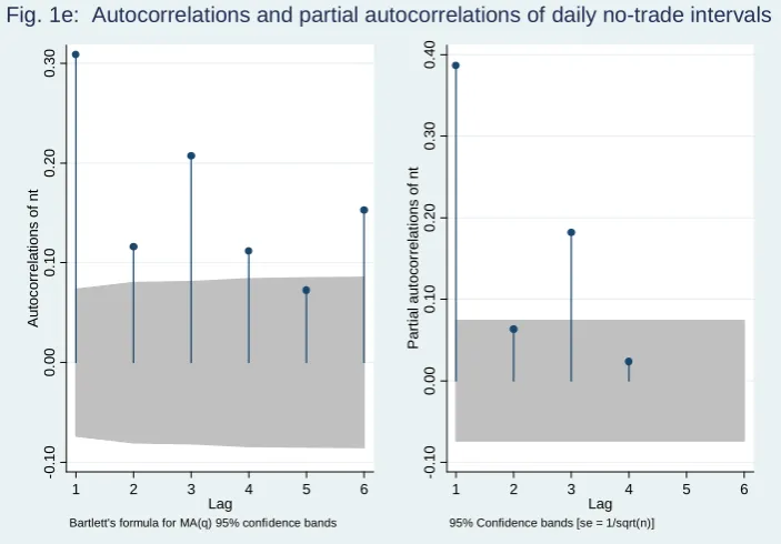
Finally, autocorrelation and partial autocorrelation of the random

vari-ables number of daily buys on MTS (BQ), number of daily buys on

BondVi-sion (BO), number of daily sells on MTS (SQ), number of daily sells (SO) on

BondVision and number of no trade days (NT), show that there is persistence

in the data. However, Easley and O’Hara (1992) argue that dependence does

not affect the estimates ofµand, because they are determined by the

num-ber of trades and no trades occurred within a trading day. Nonetheless, the

estimates ofα andδ may be affected since they are derived from the

distri-bution of trades and no trades between days. Details of the autocorrelations

and partial autocorrelations for six lags are reported in Appendix C.

7

Conclusions

In this paper we investigate the presence of asymmetric information in the

two secondary government bond market. We analyse the parallel trading of

fixed rate bond (BTP) with a ten-year maturity on two secondary electronic

Our model allows to explain the stochastic process governing the asset

prices on the base of the number of buys, sells and no trade intervals occurred

over a sample of 708 days.

Asymmetric information arises since each day nature deliver a signal to

the market about the true value of the asset. This signal could be good or

bad and it is delivered only to a fraction of traders (informed traders).

The dataset allows us to know exactly the type of trades occurred, i.e. if

it is a buy or a sell. This is a remarkable advantage compared to works that

use anad-hoc algorithm to infer this piece of information, introducing noise

in the results.

The two platforms under analysis differ for the degree of transparency

that typifies them. We assume that the probability to encounter an informed

trader on the less transparent market is higher than the corresponding

prob-ability on the more transparent one. Our results confirm this assumption,

since informed traders on MTS are 18 per cent, whereas on BondVision, the

less transparent platform, they are 31 per cent. Although our theoretical

model is constructed to include both platforms, the value of the estimates

that we obtain from the two separate markets are still informative.

Furthermore, we perform a series of robustness tests.

First we check for the robustness of our estimates to different lengths of

the trade intervals. We estimate the maximum log-likelihood also for time

intervals of 8 and 10 minutes, and we do not find any significant difference.

Second we perform a non-parametric run test to asses the independence

of information events form day to day. This test rejects the null hypothesis

of independence. However this finding does not controvert the hypothesis of

our model, but calls for further analysis, in order to relax the assumption

auto-correlated or cross-auto-correlated.

Finally, we investigate the presence of autocorrelation and partial

auto-correlation in the random variables of our model. Also in this case the results

are not respondent to the hypothesis of no dependence, calling for further

Appendix A

Table 7: 8-min intervals (MTS platform)

Parameter Coef. Std. Err. Z P > |Z| 95% Conf. Interval

α .3804801 .0024091 157.94 0.000 .3757584 .3852017 δ .5523178 .0038858 142.14 0.000 .5447017 .5599338 µ .2438671 .0004279 569.90 0.000 .2430284 .2447058 .562448 .000214 2627.98 0.000 .5620285 .5628675

Log-likelihood = -8228512.2

Table 8: 8-min intervals (BondVision platform)

Parameter Coef. Std. Err. Z P > |Z| 95% Conf. Interval

α .3942688 0027373 144.04 0.000 .3889038 .3996338 δ .6823738 .0038475 177.36 0.000 .6748329 .6899147 µ .1551226 .0004542 341.55 0.000 .1542325 .1560128 .1607788 .0002514 639.44 0.000 .160286 .1612716

Log-likelihood = -2454951.8

Table 9: 10-min intervals (MTS platform)

Parameter Coef. Std. Err. Z P > |Z| 95% Conf. Interval

α .3804801 .0026589 143.10 0.000 .3752687 .3856914 δ .5523178 .0042888 128.78 0.000 .5439118 .5607237 µ .2438671 .0004723 516.25 0.000 .2429414 .2447928 .562448 .0002362 2381.04 0.000 .561985 .562911

Log-likelihood = -6754748.9

Table 10: 10-min intervals (BondVision platform)

Parameter Coef. Std. Err. Z P > |Z| 95% Conf. Interval

α .3942688 .0030212 130.50 0.000 .3883474 .4001902 δ .6823738 .0042465 160.69 0.000 .6740508 .6906968 µ .1551226 .0005013 309.45 0.000 .1541401 .1561051 .1607788 .0002775 579.35 0.000 .1602349 .1613227

Appendix B

For a trade at timet we have:

P{Ψ =H|θ1, . . . θt−1, SQ,t}=

P{Ψ =H|θ1, . . . θt−1} ·P{SQ,t|θ1, . . . θt−1,Ψ =H} P{SQ,t|θ1, . . . θt−1}

where the probability of a sale on the quote-driven platform, given(θ1, . . . θt−1)

is:

P{SQ,t|θ1, . . . θt−1}=

P{Ψ =H|θ1, . . . θt−1} ·β(1−µQ)Q(1−η)

+P{Ψ =L|θ1, . . . θt−1} ·βµQ+β(1−µQ)Q(1−η)

+P{Ψ = 0|θ1, . . . θt−1} ·βQ(1−η)

The market maker’s ask and bid in period t are given by expected value of

the asset conditional on the history and, a buy or a sell respectively.

aQ,t=E[V|BQ,t] =

V ·P{Ψ =L|θ1, . . . θt−1, BQ,t}

+V ·P{Ψ =H|θ1, . . . θt−1BQ,t}

bQ,t=E[V|SQ,t] =

V ·P{Ψ =L|θ1, . . . θt−1, SQ,t}

+V ·P{Ψ =H|θ1, . . . θt−1SQ,t}

Appendix C

Figure 4: Autocorrelations and partial autocorrelations of daily no-trade intervals

-0

.1

0

0.

00

0.

10

0.

20

0.

30

A

u

to

c

o

rr

el

at

ions

of

nt

1 2 3 4 5 6

Lag

Bartlett's formula for MA(q) 95% confidence bands

-0

.1

0

0.

00

0.

10

0.

20

0.

30

0.

40

P

a

rt

ia

l

aut

oc

or

rel

a

ti

ons

of

nt

1 2 3 4 5 6

Lag 95% Confidence bands [se = 1/sqrt(n)]