Comparison between Different Classification Methods
with Application to Skin Cancer
Yogendra Kumar Jain
HOD Computer Science & Engineering Department
Samrat Ashok Technological Institute Vidisha, (M.P), India
Megha Jain
Computer Science & Engineering Department Samrat Ashok Technological Institute
Vidisha, (M.P), India
ABSTRACT
In recent years, skin cancer is the most common form of human cancer. It is estimated that over 1 million new cases occur annually. In order to detect skin cancer various methods have been proposed in the past decades. This paper focuses on the development of a skin cancer screening system that can be used in a general practice by non-experts to classify normal from abnormal cases. The development process consists of Feature Detection and Classification Technique. The features are extracted by decomposing images into different frequency sub-bands using wavelet transform. The output of Discrete Wavelet Transform becomes input to the Classification System which classify whether the input image is cancerous or noncancerous. The classification system is based on the application of Probabilistic Neural Network and Clustering Classifier. The Accuracy of the proposed system is calculated using different classification techniques on image database of 80 samples (40 cancerous and 40 non cancerous images).
Keywords
Object Detection, Contour Tracing Algorithm, Feature Extraction, Discrete Wavelet Transform, Probabilistic Neural Network, Clustering Classifier.
1. INTRODUCTION
Skin cancer is the most common type of cancer in the United States. Since 1973, the number of new cases of melanoma, the skin cancer with the highest risk for mortality and one of the most common cancers among young adults, has increased. The incidence of melanoma has increased 150%, and melanoma mortality rates have increased by 44%. Because a substantial percentage of lifetime sun exposure occurs before age 20 years [1, 2], and ultraviolet (UV) radiation exposure during childhood and adolescence plays an important role in the development of skin cancer [1, 3].
The body is made up of different types of cells that normally divide and multiply in an orderly way. These new cells replace older cells. In case of cancer, certain cells in the body have changed in appearance and function. They divide and grow in an uncontrolled way causing cancer. Skin cancer is a disease where malignant cells are found in the epidermis (outer layer of the skin). Skin cancers can develop due to a continuous exposure to sun over the years.
Skin neoplasm (also known as “skin cancer”) is skin growths with differing causes and varying degrees of malignancies. The three most common malignant skin cancers are basal cell cancer, squamous cell cancer, and melanoma, each of which is named after the type of skin cell from which it arises. Skin cancer generally develops in the epidermis (the outermost layer of skin), so a tumor can usually be seen. This means that it is often possible to detect skin cancers at an early stage. Unlike
many other cancers, including those originating in the lung, pancreas, and stomach, only a small minority of those affected will actually die of the disease, though it can be disfiguring. Melanoma survival rates are poorer than for non-melanoma skin cancer, although when melanoma is diagnosed at an early stage, treatment is easier and more people survive.
This paper proposes a new approach for skin cancer classification by which we can detect features of a digital image and also classify that whether the given input image is cancerous or noncancerous. We are using Discrete Wavelet Transform for feature detection and classification methodology is based on Probabilistic Neural Network and Clustering Classifier.
2. LITERATURE SURVEY
The work presented in this paper is focused on the development of skin cancer detection and classification in digital images. In this paper, Vigorous research has been pursued in skin cancer detection for a number of years. In the area of skin cancer detection and classification system different technologies have been used and still the area is being explored. In this section we review some of the papers on skin cancer detection and classification. The approaches used by different researchers differ in the type of features extracted, the training method, and the classification model used.
In 1993, Ercal proposed a simple and effective technique to find the borders of tumors in color images. The method makes use of an adaptive color metric from the red, green, and blue (RGB) planes that contain information to differentiate the tumor from the background. Using this suitable coordinate transformation, the image is segmented and the tumor portion is then extracted from the segmented image and borders are drawn [4].
In 1997, Jackowskia presented an automatic method for segmentation of images of skin cancer and other pigmented lesions. This method first reduces a color image into an intensity image and approximately segments the image by intensity thresholding. Then, it refines the segmentation using image edges. Double thresholding is used to focus on an image area where a lesion boundary potentially exists. Image edges are then used to localize the boundary in that area. A closed elastic curve is fitted to the initial boundary, and is locally shrunk or expanded to approximate edges in its neighborhood in the area of focus [5].
additional preprocessing step. Following these steps, the skin lesion is segmented either by the geodesic active contours model or the geodesic edge tracing approach [6].
In 2003, Berrar presented a Gene expression profiling by microarray technology has been successfully applied to classification and diagnostic prediction of cancers. Various machine learning and data mining methods are currently used for classifying gene expression data. However, these methods have not been developed to address the specific requirements of gene microarray analysis. First, microarray data is characterized by a high-dimensional feature space often exceeding the sample space dimensionality by a factor of 100 or more. In addition, microarray data exhibit a high degree of noise. Most of the discussed methods do not adequately address the problem of dimensionality and noise. Furthermore, although machine learning and data mining methods are based on statistics, most such techniques do not address the biologist’s requirement for sound mathematical confidence measures. Finally, most machine learning and data mining classification methods fail to incorporate misclassification costs, i.e. they are indifferent to the costs associated with false positive and false negative classifications. This paper presents a probabilistic neural network (PNN) model that addresses all these issues. The PNN model provides sound statistical confidences for its decisions, and it is able to model asymmetrical misclassification costs. Furthermore, they demonstrate the performance of the PNN for multiclass gene expression data sets and compare the performance of the proposed PNN model with two machine learning methods, a decision tree and a neural network. To assess and evaluate the performance of the classifiers, they use a lift-based scoring system that allows a fair comparison of different models. The PNN clearly outperformed the other models. The results demonstrate the successful application of the PNN model for multiclass cancer classification [7].
In 2004, Sigurdsson devised a Skin lesion classification based on in vitro Raman spectroscopy is approached using a nonlinear neural network classifier. The classification framework is probabilistic and highly automated. The framework includes a feature extraction for Raman spectra and a fully adaptive and robust feed forward neural network classifier. Moreover, classification rules learned by the neural network may be extracted and evaluated for reproducibility, making it possible to explain the class assignment [8].
In 2009 Madasu and Lovell presented a ‘Fuzzy Co-Clustering Algorithm for Images (FCCI)’ technique and have been successfully applied to color segmentation of medical images. The goal of this work is to extend this technique by the inclusion of texture features as a clustering parameter for detecting blotches in skin lesions based on color information. The objective function is optimized using the bacterial foraging algorithm which gives image specific values to the parameters involved in the algorithm [9].
In 2011 Ganzeli proposed a system named as SKAN: Skin Scanner – System for Skin Cancer Detection Using Adaptive Techniques – combines computer engineering concepts with areas like dermatology and oncology. Its objective is to discern images of skin cancer, specifically melanoma, from others that show only common spots or other types of skin diseases, using image recognition. This work makes use of the ABCDE visual rule, which is often used by dermatologists for melanoma identification, to define which characteristics are analyzed by the software. It then applies various algorithms and techniques, including an ellipse-fitting algorithm, to extract and measure
these characteristics and decide whether the spot is a melanoma or not [10].
In 2011 Wei Xu presented anImage analysis of cancer cells is important for cancer diagnosis and therapy, because it recognized as the most efficient and effective way to observe its proliferation. For the purpose of adaptive and accurate cancer cell image segmentation, a double threshold segmentation method is proposed. Based on a single gray-value histogram of the RGB color space, a double threshold, the key parameters of threshold segmentation can be fixed by a fitted-curve of the RGB component histogram. As reasonable thresholds confirmed binary segmentation dependent on two thresholds, will be put into practice and result in binary image. With the post-processing of mathematical morphology and division of whole image, the better segmentation result can be finally achieved. By the comparison with other advanced segmentation methods such as level set and active contour, the proposed double thresholding has been found as the simplest strategy with shortest processing time as well as highest accuracy. The proposed method can be effectively used in the detection and recognition of cancer stem cells in images [11]
In 2011 Mahmoud proposed an automatic skin cancer (melanoma) classification system. The input for the proposed system is a collected data image, it followed by different image processing procedures to enhance the image properties. Two segmentation methods used to identify the normal skin cancer from malignant skin and to extract the useful information from these images that passed to the classifier for training and testing. The features used for classification is the coefficients created by Wavelet decompositions and simple wrapper curve let [12].
In 2011 Blackledge presented an overview of a new web-based technology for skin cancer screening. The technology is based on an expert system designed to classify moles through an analysis of a good quality digital image uploaded by the user of the system. The technology is an example of an intensive application and service in the area of Health Informatics and has been developed as a personalized e-Health Service [13].
3. BACKGROUND THEORY
3.1Feature
detection
Using
Wavelet
Transform:
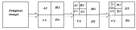
In numerical analysis and functional analysis, a Discrete Wavelet Transform (DWT) is any wavelet transform for which the wavelets are discretely sampled. As with other wavelet transforms, a key advantage it has over Fourier transforms is temporal resolution: it captures both frequency and location information (location in time).Wavelet can be implemented as a filter bank that use high pass filter g and low pass filter h to decompose 1D (signal) or 2D (image) into some chosen frequency sub bands along the rows of the signal and along the rows and columns in image. Wavelet decomposition of a two dimensional signal can be computed as shown in Fig.1. It illustrates the decomposition of the image A2j+1f into A2jf, Dh2jf, Dv2jf and Dd2jf in the frequency domain. The imagesA2j+1f, A2jf, Dh2jf, Dv2jf and Dd2jf corresponding to the lowest frequencies, the vertical high frequencies (horizontal edges), the horizontal high frequencies (verticaledges) and the high frequencies in both directions(Diagonal) respectively. i.e., the image A2
j+1 f = A2
j f + Dh2
j f + Dv2
j f + Dd2
j
f this set of images is called an orthogonal wavelet representation in two dimensions [14]. The image A2
j
f is the coarse approximation at the resolution 2j, and the images Dh2jf, Dv2jf and Dd2jf give the detail signals for different orientations and resolutions Dh2
Fig 1: A wavelet decomposition of image
Wavelets decompose an image into orthogonal sub bands with low–low (LL), low–high (LH), high–low (HL), and high–high (HH) components which Correspond to approximation, horizontal, vertical and diagonal respectively. The LL sub-band is further decomposed into another four sub-sub-bands; and
[image:3.595.177.415.325.378.2]the Low–low–low–low (LLLL) component, which represents the image approximation at this level, is decomposed once again and so on [15]. Figure.2 illustrates three levels multiresolution decomposition wavelet.
Fig 2: Three levels multiresolution decomposition wavelet
3.2Object Classification:
In order to classify an image
two classification methods Probabilistic Neural Network and Clustering Classifier are described as follows:
3.2.1 Using Probabilistic Neural Network:
A Probabilistic Neural Network (PNN) is a feed forward neural network, which was derived from Bayesian network and a statistical algorithm called Kernel Fisher discriminant analysis. It was introduced by D.F. Specht in the early 1990s [8]. In a PNN, the operations are organized into a multilayered feed forward network with four layers: Input layer Hidden layer
Pattern layer/Summation layer Output layer
The operation of the basic PNN is best shown on a simple architecture as depicted in Figure 3. The input layer of the PNN as shown in figure contains two input neurons, NI1 and NI2, for the two test cases, Xr and Yr. The pattern layer contains one pattern neuron for each training case, with an exponential activation function. A pattern neuronNi computes the squared Euclidean distance between a new input vector Xr and the i-th training vector of the j-th class. This distance is then transformed by the neuron’s activation function.
In the PNN of Figure 3, the training set comprises cases belonging to two classes, A and B. In total, m training cases belong to class A. The associated pattern neurons are N1…Nm. For example, the neuron N3 contains the third training case of class A. Class B contains n – m training cases; the associated pattern Neurons are Nm+1…Nn. For example, the neuron Nm+2 contain the second training case of class B. For each class, the summation layer contains a summation neuron. Since we have two classes in this example, Neurons are Nm+1…Nn. The PNN has two summation neurons. The summation neuron for class A
sums the output of the pattern neurons that contain the training cases of class A. The summation neuron for class B sums the output of the pattern neurons that contain the training cases of class B. The activation of the summation neuron for a class is equivalent to the estimated density function value of this class. The summation neurons feed their result to the output neurons in the output layer. These neurons are threshold discriminators that implement Bayes’ decision criterion.
The output neuron NO1 generates two outputs: the estimated conditional probability that the test case Xr belongs to class A, and the estimated conditional probability that this case belongs to class B. The output neuron NO2 generates the respective estimated probabilities for the test case Yr. Unlike other feed-forward neural networks, e.g., multi-layer perceptron (MLPs), all hidden-to-output weights are equal to 1 and do not vary during processing.
Fig 3: Architecture of a four-layered PNN for n training cases of 2 classes
…. ….
…
…..
………..
Output layer
Summation layer
Pattern layer
Input layer
Rows Columns
HH HL LH LL
h ↓2
↓2
h
g
↓2
↓2
h
g
↓2
↓2 g
A2j+1f
Low pass filtered version of the image
[image:3.595.310.539.588.732.2]3.2.2 Using Clustering Classifier:
The Clustering classifier group’s data instances into subsets in such a manner that similar instances are grouped together, while different instances belong to different groups. The instances are thereby organized into an efficient representation that characterizes the population being sampled. Formally, the clustering structure is represented as a set of subsets C =C1… Ck of S, such that: S = ⋃ I and Ci ⋂ j =ɸ for i ≠ j. Consequently, any instance in Sbelongs to exactly one and only one subset [11].
The simplest and most commonly used algorithm, employing a squared error criterion is the K-means algorithm. This algorithm partitions the data into K clusters (C1, C2……CK), represented by their centers or means. The center of each cluster is calculated as the mean of all the instances belonging to that cluster. Algorithm to classify or to group our objects based on attributes/features into K number of group. K is positive integer number. The grouping is done by minimizing the sum of squares of distances between data and the corresponding cluster centroid. Thus, the purpose of K-mean clustering is to classify the data.
Then the K means algorithm will do the three steps below until convergence:
Iterate until stable (= no object move group):
1. Determine the centroid coordinate
2. Determine the distance of each object to the centroid
3. Group the object based on minimum distance (find the closest centroid)
4. PROPOSED METHODOLOGY
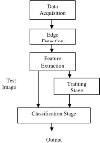
[image:4.595.326.531.321.370.2]The flowchart for the proposed system is shown in figure 4. Initially, browse the input image and the edges of each input image are detected using Contour Tracing Algorithm. Then the output of edge detection becomes input to the Discrete Wavelet Transform which decomposed image and produced approximation coefficients, then classifies image using different classification methods and compare the result based on certain parameters.
Fig 4: Proposed System
4.1 Image Acquisition
:
The database images used, contains both digital photo and dermoscopy images. These images were collected from different sources. Total 80 images are collected; these images include digital cancerous images and digital non cancerous images. These images separated into two groups to test the accuracy of each group. The database images are obtained from different sources and the size of the images is non-standard. The first step in the process is to resize the image to have a fixed width and height. [image:4.595.87.248.506.735.2]4.2 Edge Detection
:
Edge detection is an important task in image processing. It is a main tool in pattern recognition, image segmentation, and scene analysis. An edge detector is basically a high pass filter that can be applied to extract the edge points in an image. Edges characterize object boundaries and are therefore, useful for segmentation, registration, and identification of objects in scenes. In this paper for detecting the edges of an image contour tracing algorithm is used which is same as previous work. In order to detect the edges of an image imcontour () function is used. Imcontour (I, n) draws a contour plot of the grayscale image I, automatically setting up the axes so their orientation and aspect ratio match the image n is the number of equally spaced contour levels in the plot. Figure 5 demonstrates the edge detection of an image:Fig 5: Edge detection of Cancerous image
4.3 Discrete Wavelet Transform
:
A modern method of feature extraction, discrete wavelet transformation which is discussed and used in this paper. One of the most powerful computing methods these system use is the multiresolution analysis of digitized images, based on wavelet transform. Before applying wavelet transform, the image need to be convert into negative image based on the concept that the lower frequency will transform to the higher frequency domain and vice versa. The detection of cancer was achieved by decomposing the input image into different frequency sub-bands. Then extract the value of approximation coefficient from the decomposed image. After that reconstructing the decomposed image from the sub-bands containing only low frequencies and this value becomes input to the neural network classifier. Figure 6 shows the various wavelet transformation steps:Fig 6: Wavelet Transform steps Preprocessed image
Negative image
Approximation Coefficient
Reconstruction
Cancer Detection Wavelet Transform Data
Acquisition
Edge Detection
Training Stage
Classification Stage Test
Image
[image:4.595.357.494.565.746.2]Wavelet decomposition can be a repeated process occurring over several levels. The original signals are decomposed into approximations feeding the next level of decomposition, creating a decomposition tree. In this stage, multilevel 2-D wavelet decomposition on the input image is performed. It is performed by using Wavelet filters and Outputs are the decomposition vector. Then the discrete 2-D wavelet transform on the decomposed image is calculated and compute the approximation coefficients matrix cA and details coefficients matrices say, cH, cV, and cD (horizontal, vertical, and diagonal, respectively), and the values of coefficient matrix are stored in an array say [cA cH cV cD]. The approximation and details coefficients are stored in one big 2D array is as follows:
(cA, (cH, cV, cD))
LL Sub band contains all wavelet coefficients those results from applying low pass filter to both rows and columns of an image.
HL Sub band consists of all wavelet coefficient results from low pass filtering of the rows, followed by high filtering of the columns.
LH Sub band consists of all wavelet coefficient results from high pass filtering of the rows ,followed by low pass filtering of the columns , and mostly it Carries information about the vertical details or edges.
HH Sub band consists of all wavelet coefficient results from applying high pass filter to both rows by high and columns. This usually captures the diagonal edges or details of the original images.
[image:5.595.101.241.531.634.2]Further, the coefficients that are neglected during approximation are cH, cV, and cD. The value of approximation coefficient cA is extracted from the decomposed image and stored in an array named as, feature_vect.and this becomes input to PNN. Figure, shows the Discrete Wavelet Transform of cancerous image using Haar Wavelet
Fig 7: Decompose input image using Discrete Wavelet Transform
4.4 Decision Making System:
For classification of skin cancer two different classification methods are used and they are as follows:4.4.1 Neural Networks Classifier
:
A Probabilistic Neural Network is used to identify whether the image is cancerous or not. In order to classify an image using PNN two class s1 and s2 are used. Class s1 contains cancerous images while Class s2 contains noncancerous images. The classification systemclassifies whether the input image belongs to s1 class or s2 class.
The extracted approximation coefficient is considered as input to the neural classifier. A probabilistic neural network is a set of connected input/output units in which each connection has a weight associated with it. The PNN trained by adjusting the weights so as to be able to predict the correct class. The desired output was specified as 1 for normal and 0 for abnormal. The classification process is divided into the training phase and the testing phase. In the training phase known data are given, the proposed system is trained using 80 data sets. In the testing phase, unknown data are given and the classification is performed using the classifier after training. The ability of the classifier to assign the unknown object to the correct class is dependent on the extracted features, and the accuracy of the classification depends on the efficiency of the training.
4.4.2 Clustering classifier:
The second classification method which is used to classify whether the input image is cancerous or not isClustering Classifier. In order to identify an image by clustering classifier the clusters are used, which group the set of objects so that the objects in the same cluster are more similar (in some sense or another) to each other than to those in other clusters. The proposed system used a Centroid Based Clustering Algorithm for classification of skin cancer images.In centroid-based clustering, clusters are represented by a central vector which may not necessarily be a member of the data set. Here the number of clusters is fixed to 2 because we have only two types of images that are cancerous and non-cancerous. In centroid based clustering classification initially, we extract the value of feature_vect from Discrete Wavelet Transform, calculate the mean value and find the cluster centers and assign the objects to the nearest cluster center, such that the squared distances from the cluster are minimized. The classification process is divided into the training phase and the testing phase. In the training phase known data are given, the proposed system is trained using 80 data sets. In the testing phase, unknown data are given and the classification is performed using the clustering classifier after training.
5. RESULT AND DISCUSSION
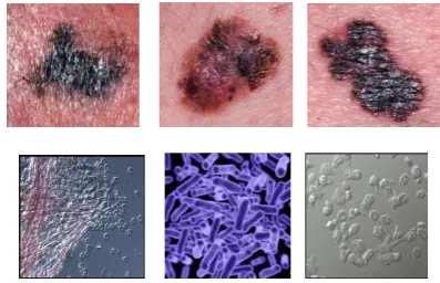
The proposed system was implemented in MATLAB and tested on various Skin Cancer images. In our database 80 images are included, in that 40 images belong to cancerous class and 40 belong to non cancerous class. Some of the samples from the database are as follows:
Fig 8: Samples of Cancerous and Non Cancerous images
For each input image Feature Vector is calculated and classifies the input image using different classification methods i.e. Probabilistic Neural Network and clustering Classifier.
cA(LL) cH(LH)
[image:5.595.325.524.575.703.2]Parameters evaluated to measure the performance of different classifiers are as follows: (I) TPR (True Positive Rate) (II) TNR (True Negative Rate) (III) FPR (False Positive Rate) (IV) FNR (False Negative Rate) (V) ACC (Accuracy). The above parameters can be calculated as:
(TPR) = =
(FPR) =
=
(TNR) = =
(FNR) =
=
(ACC) =
The main objective of the proposed system is to obtain a high value of true positive rate and a low value of false positive rate. The term True Positives (TP's) describe, the Cancerous image that is classified by the proposed system as cancerous, and the term False Positives (FP's) describe, the image that is classified by the proposed system as cancerous image, but in fact it is not a cancerous image, the true cancerous image that is missed by the proposed system are called False Negatives (FN's), and the True Negatives (TN's) refer to the non-cancerous image that is classified by the proposed system correctly.
For different database size, the performance parameters TPR, TNR, FPR, FNR and ACC are evaluated using probabilistic neural network technique and clustering classifier.
Table1: Evaluate parameters using PNN:
Total data TPR TNR FPR FNR Accuracy
5 1 1 0 0 1
10 1 1 0 0 0.99
15 1 1 0 0 0.98
20 1 1 0 0 0.98
25 1 1 0 0 0.97
30 1 1 0 0 0.97
35 0.95 0.95 0.05 0.05 0.96
40 0.95 0.95 0.05 0.05 0.95
Table2: Evaluate parameters using Clustering:
Total data TPR TNR FPR FNR Accuracy
5 1 1 0 0 1
10 1 0.9 0.1 0 0.95
15 0.933 0.933 0.066 0.066 0.933
20 0.95 0.9 0.1 0.05 0.925
25 0.92 0.92 0.08 0.08 0.92
30 0.9 0.9 0.1 0.1 0.9
35 0.914 0.943 0.057 0.086 0.929
40 0.9 0.95 0.05 0.1 0.925
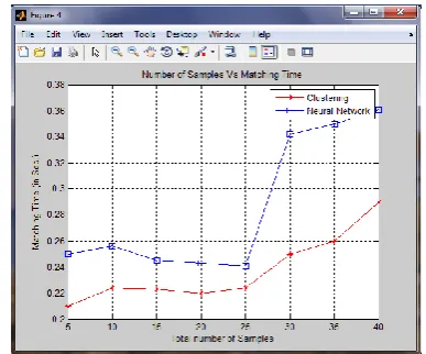
For 40 data sets the average accuracy of the proposed system using PNN is 97.5% where as it is 93.5% for Clustering Classifier. For different database size Training Time and Matching Time (Training time is the amount of time required to train the network and matching time is the amount of time required to match the input image from the data set) is
evaluated, and plot the graph between number of samples and detection accuracy, number of samples and training time, number of samples and matching time for different classification techniques i.e. Probabilistic Neural Network and Clustering Classifier.
Figure 9, demonstrate graph between number of samples and detection accuracy, the Number of Samples is taken on x-axis and Detection Accuracy is taken on y-axis. As shown in figure, the accuracy of the system decreases as the number of samples increases for both techniques i.e. Probabilistic Neural Network and Clustering Classifier. But the accuracy of Neural Network Classifier is better than Clustering Classifier.
[image:6.595.327.520.207.376.2]Fig 9: Graph Showing Number of Samples Vs Detection Accuracy
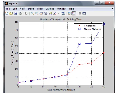
[image:6.595.330.519.485.636.2]Figure 10, demonstrates the graph between Number of Samples and Training Time, the number of samples is taken on x-axis and training time is taken on y-axis. Figure indicates that the training time for both the algorithm is same when the number of samples are less but as the number of samples increases the training time gradually increases, and the Neural Network Classifier requires more training time than Clustering Classifier.
Fig 10: Graph Showing Number of Samples Vs Training Time
[image:6.595.51.291.540.687.2]Fig 11: Graph showing Number of Samples Vs Matching Time
6. CONCLUSION
This paper presents a various methods for classification of skin cancer. The proposed system is evaluated on 80 images for classification of skin cancer using Probabilistic Neural Network and Clustering Classifier. Out of these classification methods we conclude from the results that the classification using Probabilistic Neural Network is better as compared to Clustering Classifier. This is a significant improvement as compared to the earlier techniques proposed in the same domain. PNN perform better than other types of artificial neural networks (ANNs) and have shown excellent classification performance.
In contrast to other types of ANNs, e.g. MLPs, PNN are not “black boxes”: The contribution of each pattern neuron to the outcome of the network is explicitly defined and accessible, and has a precise interpretation. The training of PNN involves no heuristic searches, but consists essentially of incorporating the training cases into the pattern layer. However, finding the best smoothing factor for the training set remains an optimization problem. PNNs tolerate erroneous samples and outliers. Sparse samples are adequate for the PNN. Other types of ANN and many traditionalStatistical techniques are hampered by outliers. Finally, when new training data become available, PNN do not need to be reconfigured or retrained from scratch; new training data can be incrementally incorporated in the pattern layer.
A disadvantage of PNNs is the fact that all training data must be stored in the pattern layer, requiring a large amount of memory. But in general, today’s standard PCs have a sufficiently large main memory capacity for an efficient implementation of PNN. In applications where large amounts of training cases are available, this argument against PNNs becomes relevant. Although the output of the PNN is probabilistic, we should keep in mind that the probabilities are estimates and conditional on the learning set.
REFERENCES
[1] Weinstock MA, Colditz GA, Willett WC, Stampfer MJ, Bronstein BR Jr, Speizer FE,”Nonfamilial cutaneous melanoma incidence in women associated with sun exposure before 20 years of age”, Pediatrics1989; 84, pp: 199–204.
[2] Stern RS, Weinstein MC,Baker SG,”Risk reduction for nonmelanoma skin cancer with childhood sunscreen use”, Arch Dermatol 1986; 122, pp: 537–45.
[3] Gilchrest BA, Eller MS, Geller AC, Yaar M,” The pathogenesis of melanoma induced by ultraviolet radiation”, N Engl J Med 1999; pp: 1341–1348.
[4] F. Ercal, “Detection of Skin Tumor Boundaries in Color Images”, IEEE Transactions on Medical Imaging, vol. 12, no. 3, September 1993, pp: 624 – 626.
[5] L. Xu, M. Jackowski, A. Goshtasby, “Segmentation of Skin Cancer Images”, Elsevier Journal of Image and Vision Computing, vol. 17, 1999, pp: 65–74.
[6] Do Hyun Chung and Guillermo Sapiro, “Segmenting skin Lesions with Partial-Differential-Equations-Based Image Processing Algorithms”, IEEE Transactions on Medical Imaging, vol. 19, July 2000, pp: 763-767.
[7] Daniel P. Berrar,”Multiclass Cancer Classification Using Gene Expression Profiling and Probabilistic Neural Networks”, Pacific Symposium on Biocomputing, vol. 8, 2003, pp: 5-16.
[8] Sigurdur Sigurdsson, “Detection of Skin Cancer by Classification of Raman Spectra”, IEEE Transactions on Biomedical Engineering, vol. 51, no. 10, October 2004, pp: 1784 – 1793.
[9] Vamsi K. Madasu & Brian C. Lovell, “Blotch Detection in Pigmented Skin Lesions using Fuzzy Co-Clustering and Texture Segmentation”, IEEE Conference on Digital Image Computing: Techniques and Applications, 2009, pp: 25 – 31.
[10]H. S. Ganzeli, “SKAN: Skin Scanner – System for Skin Cancer Detection Using Adaptive Techniques”, IEEE Latin America Transactions, vol. 9, no. 2, April 2011, pp: 206-212.
[11]Jin Wei Xu,” A double thresholding method for cancer stem cell detection” 7th international symposium on image and signal processing and analysis (Ispa 2011) September, pp: 695-699.
[12]Md. Khalad Abu Mahmoud, “The Automatic Identification of Melanoma by Wavelet and Curve let Analysis: Study Based on Neural Network Classification”, 11th
IEEE International Conference on Hybrid Intelligent Systems (HIS), Dec. 2011, pp: 680- 685.
[13]Jonathan Blackledge, Dimitri Dubovitski, “Mole test: A Web-based Skin Cancer Screening System”, Intensive
2011: The Third International Conference on Resource Intensive Applications and Services, vol: 978-1-61208-006-2, May, 2011, pp. 22 – 29.
[14]S. G. Mallat, “A Theory for Multiresolution Signal Decomposition: The Wavelet Representation”, IEEE Transactions on Pattern Analysis and Machine Intelligence vol. 7, no. 11, 1989, pp. 674–93.
[image:7.595.72.266.70.231.2]