Experimental Comparison of Different Problem
Transformation Methods for Multi-Label Classification
using MEKA
Hiteshri Modi
ME-CSE Student, Dept. of Computer Engineering Kalol Institute of Technology and Research Center
Kalol, Gujarat, India
Mahesh Panchal
Head & Associate Prof., Dept. of Computer Engg. Kalol Institute of Technology and Research Center
Kalol, Gujarat, India
ABSTRACT
Classification of multi-label and multi-target data is challenging task for machine learning community. It includes converting the problem in other easily solvable form or extending the existing algorithms to directly cope up with multi-label or multi-target data. There are several approaches in both these category. Since this problem has many applications in image classification, document classification, bio data classification etc. much research is going on in this specific domain. In this paper some experiments are performed on real multi-label datasets and three measures like hamming loss, exact match and accuracy are compared of different problem transformation methods. Finally what is effect of these results on further research is also highlighted.
General Terms
Single-label Classification, Multi-label Classification
Keywords
Binary Relevance, Label Power-Set, Label Ranking, MEKA, Multi-Label Ranking, Pruned Set
1.
INTRODUCTION
Single label classification is one in which training examples are associated with only one label from a set of disjoint labels. But applications such as text categorization, semantic scene classification, music categorization may belong to more than one class. These applications require multi-label classification. In multi-label classification training examples are associated with more than one label from a set of disjoint labels. For example, in medical diagnosis a patient may suffer from diabetes and cancer both at the same time.
Two main methods of multi-label classification exists: The first one is Problem Transformation(PT) Method, in which multi-label classification problem is transformed into single-label classification problem and then classification is performed in the same way as in single-label classification process. The second method is Algorithm Adaptation Method, in which existing single-label classification algorithms are modified and then applied directly to multi-label data. The main focus of this paper is on Problem Transformation Method. Various problem transformation methods exists in different literatures such as simple problem transformation methods(copy, copy-weight, max, min, select-random, ignore), Binary Relevance, Label Power-Set method(also known as Label Combination), Pruned Problem Transformation Method(also known as Pruned Set), Random k-label sets, Ranking by Pairwise Comparison, Calibrated Label Ranking. Algorithm Adaptation Method has also
various methods available in different literature and is discussed in brief in this paper.
There are number of evaluation measures available for multi-label classification. From them three measures: Accuracy, Hamming Loss and Exact-Match are used in this paper to evaluate different PT methods. Accuracy gives the percentage of data predicted correctly. Hamming loss gives the percentage of data predicted incorrectly on average. Exact-match gives percentage of test dataset predicted exactly same as in the training dataset. The experiments are performed using a tool, MEKA (Multi-label Extension to WEKA). MEKA has no GUI support and it is written in JAVA. MEKA supports various methods of multi-label classification.
Using experiments, in this paper, performance of three PT methods (BR, LC and PS) are compared using four different base classifiers (ZeroR, Naive Bayes, J48, JRip) against three evaluation measures described above. The experiment results indicate that LC and PS are better methods than BR.
The rest of the paper is organized as follows. Section 2 describes tasks related to multi-label classification and some examples of multi-label classification. Section 3 describes two main methods used for multi-label classification. Section 3.1 discusses various Problem Transformation methods and section 3.2 discusses various Algorithm adaptation Methods. Section 4 describes experimental studies, in which section 4.1 describes evaluation metrics used, section 4.2 describe benchmark datasets used, section 4.3 describes about tool used for experiments (MEKA) and section 4.4 gives results and discussion of experiments performed. Section 5 presents conclusion and future work.
2.
CLASSIFICATION
Classification is an important theme in data mining. Classification is a process to assign a class to previously unseen data as accurately as possible. The unseen data are those records whose class value is not present and using classification, class value is predicted. In order to predict the class value, training set is used. Training set consists of records and each record contains a set of attributes, where one of the attribute is the class. From training set a classifier is created. Then that classifier’s accuracy is determined using test set. If accuracy is acceptable then and only then classifier is used to predict class value of unseen data.
Classification can be divided in two types: single-label classification and multi-label classification
class labels L. Multi-label classification is to learn from a set of instances where each instance belong to one or more classes in L. For example, a text document that talks about scientific contributions in medical science can belong to both science and health category, genes may have multiple functionalities (e.g. diseases) causing them to be associated with multiple classes, an image that captures a field and fall colored trees can belong to both field and fall foliage categories, a movie can simultaneously belong to action, crime, thriller, and drama categories, an email message can be tagged as both work and research project; such examples are numerous[1]. In text or music categorization, documents may belong to multiple genres, such as government and health, or rock and blues [2, 3].
There exist two major tasks in supervised learning from multi-label data: multi-multi-label classification (MLC) and multi-label ranking (LR). MLC is concerned with learning a model that outputs a bipartition of the set of labels into relevant and irrelevant with respect to a query instance. LR on the other hand is concerned with learning a model that outputs an ordering of the class labels according to their relevance to a query instance.
Both MLC and LR are important in mining multi-label data. In a news filtering application for example, the user must be presented with interesting articles only, but it is also important to see the most interesting ones in the top of the list. So, the task is to develop methods that are able to mine both an ordering and a bipartition of the set of labels from multi-label data. Such a task has been recently called multi-label ranking (MLR) [4].
Multi-target classification, in which each record has multiple class-labels and each class-label, contains multiple values. Multi-label classification is one in which each record has multiple class-labels, but each class-label contains only binary values. It is a special-case of multi-target classification.
3.
METHODS FOR MULTI-LABEL
CLASIFICATION
Multi-label classification methods can be grouped in two categories as proposed in [1]:
(1) Problem Transformation Method (2) Algorithm Adaptation Method
First method transform multi-label classification problem into one or more single-label classification problem. It is algorithm independent method. Second method extends existing specific algorithm to directly handle multi-label data.
3.1
Problem Transformation Method
[image:2.595.320.550.355.462.2]All Problem transformation Methods will be exemplified through the multi-label example dataset of Table-I. It consists of five instances which are annotated by one or more out of five labels, L1, L2, L3, L4, and L5. To describe different methods, attribute field is of no important, so it is omitted in the discussion.
Table 1. Example of multi-label dataset
3.1.1
Simple Problem transformation Methods
There exist several simple problem transformation methods that transform multi-label dataset into single-label dataset so that existing single-label classifier can be applied to multi-label dataset.The Copy Transformation method replaces each multi-label instance with a single class-label for each class-label occurring in that instance. A variation of this method, dubbed copy-weight, associates a weight to each produced instances. These methods increase the instances, but no information loss is there.
The Select Transformation method replaces the Label-Set (L) of instance with one of its member. Depending on which one member is selected from L, there are several versions exist, such as, select-min (select least frequent label), select-max (select most frequent label), select-random (randomly select any label). These methods are very simple but it loses some information.
The Ignore Transformation method simply ignores all the instances which has multiple labels and takes only single-label instances in training. There is major information loss in this method.
[image:2.595.318.539.617.697.2]All simple problem transformation method does not consider label dependency. (Fig. 1)
Figure 1: Transformation of dataset of Table-1 using Simple Problem Transformation Methods
3.1.2
Binary Relevance (BR)
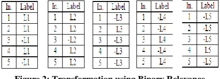
A Binary Relevance [2] is one of the most popular transformation methods which learns q binary classifiers (q=│L│, total number of classes (L) in a dataset), one for each label. BR transforms the original dataset into q datasets, where each dataset contains all the instances of original dataset and trains a classifier on each of these datasets. If particular instance contains label Lj (1≤ j ≤ q), then it is labeled positively otherwise labeled negatively. Fig. 2 shows dataset that are constructed using BR for dataset of Table I.
Figure 2: Transformation using Binary Relevance
From these datasets, it is easy to train a binary classifier for each dataset. For a new instance to classify, BR outputs the union of the labels that are predicted positively by the q classifiers.BR is used in many practical applications, but it Instance Attribute Label Set
1 A1 { L1,L2 }
2 A2 { L1,L2,L3 }
3 A3 { L4 }
4 A4 { L1, L2, L5 }
[image:2.595.93.250.671.739.2]can be used only in applications which do not hold label dependency in the data. This is the major limitation of BR.
3.1.3
Label Power-Set (LP)
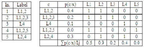
The Label Power-set method [3] removes the limitation of BR by taking into account label dependency. Label Power-set considers each unique occurrence of set of labels in multi-label training dataset as one class for newly transformed dataset. For example, if an instance is associated with three labels L1, L2, L4 then the new single-label class will be L1,2,4. So the new transformed dataset is a single-label classification task and any single-label classifier can be applied to it. (Fig. 3)
[image:3.595.319.546.250.379.2]For a new instance to classify, LP outputs the most probable class, which is actually a set of labels. Thus it considers label dependency and also no information is lost during classification. If the classifier can produce probability distribution over all classes, then LP can give rank among all labels using the approach of [4]. Given a new instance x with unknown dataset, Fig. 3 shows an example of probability distribution by LP. For label ranking, for each label calculates the sum of probability of classes that contain it. So, LP can do multi-label classification and also do the ranking among labels, which together called MLR (Multi-label Ranking) [4].
Figure 3: Transformation using Label Power-Set and Example of obtaining Ranking from LP
As stated earlier, LP considers label dependencies during classification. But, its computational complexity depends on the number of distinct label-sets that exists in the training set. This complexity is upper bounded by min(m,2q). The number of distinct label is typically much smaller, but it is still larger than q and poses important complexity problem, especially for large values of m and q. When large number of label-set is there and from which many are associated with very few examples, makes the learning process difficult and provide class imbalance problem. Another limitation is that LP cannot predict unseen label-sets. LP can also be termed as Label-Combination Method (LC) [6].
3.1.4
Pruned Problem Transformation (PPT)
The pruned problem transformation method [5] extends LP to remove its limitations by pruning away the label-sets that are occurring less time than a small user-defined threshold. That is removes the infrequent label-sets. It also optionally replaces these label-sets by disjoint subsets of those label-sets that are occurring more time than the threshold. PPT is also referred as Pruned Set (PS) [6].3.1.5
Random k-label sets (RAkEL)
The random k-label sets (RAkEL) method [2] constructs an ensemble of LP classifiers. It works as follows: It randomly breaks a large sets of labels into a number (n) of subsets of small size (k), called k-label sets. For each of them train a
multi-label classifier using the LP method. Thus it takes label correlation into account and also avoids LP's problems. Given a new instance, it query models and average their decisions per label. And also uses thresholding to obtain final model. Thus, this method provides more balanced training sets and can also predict unseen label-sets.
3.1.6
Ranking by Pairwise Comparison (RPC)
Ranking by pairwise comparison[7] transforms the multi-label datasets into q(q-1)/2 binary label datasets, one for each pair of labels (Li, Lj), 1≤i<j<q. Each dataset contains those instances of original dataset that are annotated by at least one of the corresponding labels, but not by both. (Fig. 4) [image:3.595.57.290.336.412.2]A binary classifier is then trained on each dataset. For a new instance, all binary classifiers are invoked and then ranking is obtained by counting votes received by each label.
Figure 4: Transformation using Ranking by Pairwise Comparison
3.1.7
Calibrated Label Ranking (CLR)
CLR is the extension of Ranking by Pairwise Comparison [8]. This method introduces an additional virtual label (This method introduces an additional virtual label (calibrated label), which acts as a split point between relevant and irrelevant labels. Thus CLR solves complete MLR task. Each example that belongs to particular label is considered positive for that example that does not belongs to particular label is considered negative for that particular label and positive for virtual label. Thus CLR corresponds to the model of Binary Relevance. When CLR applied to the dataset of Table I, it constructs both datasets of Fig. 4 and Fig. 2.
3.2
Algorithm Adaptation Method
3.2.1
Decision Tree based
Multi-label C4.5 [9] is an extension of popular C4.5 decision tree to deal with multi-label data. It defines “multi-label entropy” over a set of multi-label examples, based on which the information gain of selecting a splitting attribute is calculated, and then a decision tree is constructed recursively in the same way of C4.5.
Given a set of multi-label examples
Let p(y) denotes the probability that an example in S has label y, then the multi-label entropy is:
3.2.2
Tree Based Boosting
AdaBoost.MH and AdaBoost.MR [10] are two extension of AdaBoost for multi-label data. AdaBoost.MH is designed to minimize Hamming loss and Adaboost.MR is designed to find hypothesis with optimal ranking. AdaBoost.MH is extended in [11] to produce better human related classification rule.
3.2.3
Neural Network based
BP-MLL [12] is an extension of the popular back-propagation algorithm for multi-label learning. The main modification is the introduction of a new error function that takes multiple labels into account. Given multi-label training set,
The global training error E on S is defined as:
Where, Ei is the error of the network on (xi, Yi) and cij is the actual network output on xi on the jth label.
The differentiation is the aggregation of the label sets of these examples.
3.2.4
Lazy Learning
There are several methods [13, 14, 15, 16] exists based on lazy learning (i.e. k-Nearest Neighbour (kNN)) algorithm. All these methods are retrieving k-nearest examples as a first step.
ML-kNN [16] is the extension of popular kNN to deal with multi-label data. It uses the maximum a posteriori principle in order to determine the label set of the test instance, based on prior and posterior probabilities for the frequency of each label within the k nearest neighbours.
4.
EXPERIMENTAL SETUP
4.1
Evaluation Metrics
Several evaluation measures exists for multi-label classification, from them accuracy, hamming loss, exact-match are used in this literature.
4.1.1
Accuracy (A)
Accuracy for each instance is defined as the proportion of the predicted correct labels to the total number (predicted and actual) of labels for that instance. Overall accuracy is the average across all instances [17].
Accuracy A
=
4.1.2
Hamming Loss (HL)
Hamming Loss reports how many times on average, the relevance of an example to a class label is incorrectly predicted. Therefore, hamming loss takes into account the prediction error (an incorrect label is predicted) and the missing error (a relevant label not predicted), normalized over total number of classes and total number of examples. Hamming Loss is defined as follow in [10]:
Hamming Loss
=
Where ∆ stands for the symmetric difference of two sets, which is the set-theoretic equivalent of the exclusive disjunction (XOR operation) in Boolean logic.
4.1.3
Exact Match
Exact Match is defined as the accuracy of each example where all label relevancies must match exactly for an example to be correct.
4.2
Benchmark Datasets
4.2.1
Scene
The Scene dataset was created to address the problem of emerging demand for semantic image categorization. Each instance in this dataset is an image that can belong to multiple classes. This dataset has 2407 images each associated with some of the 6 available semantic classes (beach, sunset, fall foliage, field, mountain, and urban). This dataset contains 963 predictor attributes.
4.2.2
Enron
The Enron Email dataset contains 517,431 emails (without attachments) from 151 users distributed in 3500 folders, mostly of senior management at the Enron Corp.[5] After preprocessing and careful selection, a substantial small amount of email documents (total 1702) are selected as multi-label data, each email belonging to at least one of the 53 classes[3]. This dataset contains 681 predictor attributes.
4.3
Tool
The experiments are performed in MEKA which is a tool for multi-label classification. The MEKA project provides an open source implementation of methods for multi-label classification in JAVA. It is based on the WEKA machine learning toolkit from the University of Waikato. MEKA does not yet integrated with the WEKA GUI interface and is mainly intended to provide implementations of published algorithms.
4.4
Results and Discussion
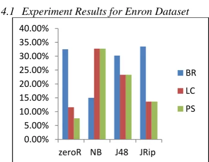
In this paper as stated earlier two datasets are used, Scene and Enron. Three PT methods are taken to compare experiment result, Binary Relevance (BR), Label Power-set (LC-Label Combination) and Pruned Problem Transformation (PS-Pruned Set). As a base classifier, four classifiers are used, zeroR, Naive Bayes (NB), J48 and JRip. The measures used are Accuracy, Hamming Loss and Exact-match.(Fig. 5 to fig. 10)
[image:4.595.323.533.561.724.2]4.4.1
Experiment Results for Enron Dataset
Figure 5: PT Method, Classifier Vs. Accuracy
0.00% 5.00% 10.00% 15.00% 20.00% 25.00% 30.00% 35.00% 40.00%
zeroR NB J48 JRip
BR
LC
Figure 6: PT Method, Classifier Vs. Hamming Loss
Figure 7: PT Method, Classifier Vs. Exact-Match
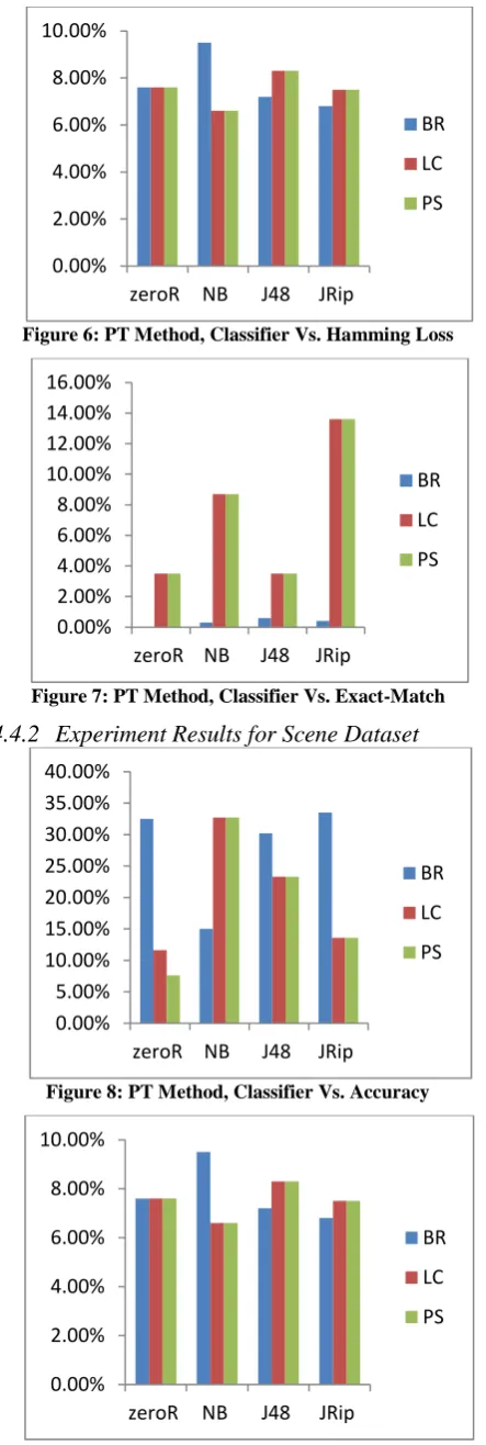
4.4.2
Experiment Results for Scene Dataset
Figure 8: PT Method, Classifier Vs. Accuracy
[image:5.595.328.541.71.220.2]Figure 9: PT Method, Classifier Vs. Hamming Loss
Figure 10: PT Method, Classifier Vs. Exact-Match
For both datasets, the result shows that when BR method is used with NB classifier, it gives more hamming loss, less accuracy and less exact-match. Whereas when LC and PS methods are used with NB classifier, it gives less Hamming loss, more accuracy and more exact-match. This is an interesting result that LC and PS give better result with NB classifier than BR.
LC and PS provide same results for these two datasets. These both methods are providing better result for both the datasets for all three measures than BR. The reason is that BR does not consider label dependency whereas LC and PS are considering label dependency and thus gives better result than BR.
5.
CONCLUSION AND FUTURE WORK
The results of experiment show that LC and PS method gives better result than BR method. The reason is that LC and PS considers label correlation during transformation from multi-label to single-multi-label dataset. Whereas BR method does not consider label correlation while transformation and thus gives less accuracy.
In this paper, main focus is on methods of multi-label classification which is a special case of multi-target classification. In the future, PS method can be extended to classify target data, since the classification of multi-target data is an open research issue.
6.
REFERENCES
[1] Tsoumakas, G., Katakis, I.: Multi-label classification: An overview. International Journal of Data Warehousing and Mining 3 (2007) 1–13
[2] Grigorios Tsoumakas, Ioannis Katakis, and Ioannis Vlahavas.: Mining Multi-label Data. O.Maimon, L. Rokach (Ed.), Springer, 2nd edition, 2010.(1-20) [3] Sorower, Mohammad S. A Literature Survey on
Algorithms for Multi-label Learning. Corvallis, OR, Oregon State University. December 2010.
[4] Brinker, K., F¨urnkranz, J., H¨ullermeier, E.: A unified model for multilabel classification and ranking. In: Proceedings of the 17th European Conference on Artificial Intelligence (ECAI ’06), Riva del Garda, Italy (2006) 489–493
[5] Read, J.: A pruned problem transformation method for multi-label classification. In: Proc.2008 New Zealand Computer Science Research Student Conference (NZCSRS 2008). (2008)143–150
[6] Classifier Chains for Multi-label Classification by : J Read
[7] H¨ullermeier, E., F¨urnkranz, J., Cheng, W., Brinker, K.: Label ranking by learning pairwise preferences. Artificial Intelligence 172 (2008) 1897–1916
0.00% 2.00% 4.00% 6.00% 8.00% 10.00%
zeroR NB J48 JRip
BR
LC
PS
0.00% 2.00% 4.00% 6.00% 8.00% 10.00% 12.00% 14.00% 16.00%
zeroR NB J48 JRip
BR
LC
PS
0.00% 5.00% 10.00% 15.00% 20.00% 25.00% 30.00% 35.00% 40.00%
zeroR NB J48 JRip
BR
LC
PS
0.00% 2.00% 4.00% 6.00% 8.00% 10.00%
zeroR NB J48 JRip
BR
LC
PS
0.00% 5.00% 10.00% 15.00%
zeroR NB J48 JRip
BR
LC
[8] Johannes F¨urnkranz, Eyke H¨ullermeier, Eneldo Lozamenc´ıa, and Klaus Brinker. Multilabel classification via calibrated label ranking. Machine Learning, 2008.
[9] Clare, A., King, R.: Knowledge discovery in multi-label phenotype data. In: Proceedings of the 5th European Conference on Principles of Data Mining and Knowledge Discovery (PKDD 2001), Freiburg, Germany (2001) 42–53
[10] Schapire, R.E. Singer, Y.: Boostexter: a boosting-based system for text categorization. Machine Learning 39 (2000) 135–168
[11] de Comite, F., Gilleron, R., Tommasi, M.: Learning multi-label alternating decision trees from texts and data. In: Proceedings of the 3rd International Conference on Machine Learning and Data Mining in Pattern Recognition (MLDM 2003), Leipzig, Germany (2003) 35–49
[12] Zhang, M.L., Zhou, Z.H.: Multi-label neural networks with applications to functional genomics and text categorization. IEEE Transactions on Knowledge and Data Engineering 18 (2006) 1338–1351
[13] Luo, X., Zincir-Heywood, A.: Evaluation of two systems on multi-class multi-label document
classification. In: Proceedings of the 15th International Symposium on Methodologies for Intelligent Systems. (2005) 161–169
[14] Brinker, K., H¨ullermeier, E.: Case-based multilabel ranking. In: Proceedings of the 20th International Conference on Artificial Intelligence (IJCAI ’07), Hyderabad, India (2007)702–707
[15] Spyromitros, E., Tsoumakas, G., Vlahavas, I.: An empirical study of lazy multilabel classification algorithms. In: Proc. 5th Hellenic Conference on Artificial Intelligence(SETN 2008) (2008)
[16] Zhang, M.L., Zhou, Z.H.: Ml-knn: A lazy learning approach to multi-label learning. Pattern Recognition 40 (2007) 2038–2048
[17] S. Godbole and S. Sarawagi. Discriminative Methods for Multi-labeled Classification. In Proceedings of the 8th Pacific-Asia Conference on Knowledge Discovery and Data Mining (PAKDD 2004), pages 22–30, 2004. [18] M. R. Boutell, J. Luo, X. Shen, and C. M. Brown.