Implementation of Taguchi Technique for Optimization of Performance Parameters of Turning Process

(1)

Implementation of Taguchi Technique for Optimization Of

Performance Parameters Of Turning Process

T. Naga Sushma

1*

_{, P. S. Naga Sree}

2

_{, Dr. Doradla Raja Ramesh}

3

1_{PG Student, Department of Mechanical Engineering, D.M.S.S.V.H College of Engineering, Machilipatnam} 2_{Assistant Professor, Department of Mechanical Engineering, D.M.S.S.V.H College of Engineering, Machilipatnam}

3_{Professor, Department of Mechanical Engineering, Sri Vasavi Institute of Engineering & Technology,} Machilipatnam, A.P., India

---*---Abstract -**

Need of industrial growth for developing

country gives rapid acceleration in the field of technical research. Industries are very much aware of producing mechanical components with good surface quality without allowing a margin of error. Among the different challenges of industry, Good surface quality of products plays vital role to thrive in the manufacturing sectors. This project attempts on optimizing various machining parameters like speed, feed, depth of cut, type of tool by Taguchi Techniques. Sixteen experimental runs based on Full Factorial Design of Taguchi method were performed. According to Grey Relational Analysis, the normalized experimental results of the performance characteristics are introduced to calculate the Coefficients and Grades. The analysis shows that the predicted values and calculated values are very close and that clearly indicates that the Taguchi GRA is an effective technique to optimize the machining parameters for turning process. Key Words: Turning, Grey Relational Analysis, Optimization, Taguchi Method, Full Factorial Design

1. INTRODUCTION

Manufacturing processes are classified into four principal types: machining, forming, casting and joining. Machining remains the most popular and easily applicable one to a large variety of material. Machining can be defined as the process of removing unwanted material from a work piece to produce the desired shape. Machining process includes five categories: turning, milling, drilling, grinding and boring. Turing is the process of machining external or internal cylindrical and conical surface. The work piece is rotated at a particular speed (cutting speed) and the tool is fed against the work piece (feed) at a certain level of engagement (depth of cut).

To ensure credible performance and prolonged service life of machinery, its components require to be manufactured with good surface finish and geometrical accuracy. Surface texture is one of the most important factors that control friction and transfer layer formation during sliding. The performance of a machined component depends to a large extent on the surface topography, hardness, nature of stress and strain induced on the surface region. Various parameters are used to evaluate surface roughness. In the present study, the arithmetic average

surface roughness Ra, root mean square Rq, skewness Rsk,

kurtosis Rku, are selected to characterize the surface

roughness as it is a key requirement for many relevant applications in industry

The Taguchi method, a well known technique that provides efficient and systematic methodology for process optimization. Taguchi method is a statistical method which was developed for the production of robust products by Professor Genichi Taguchi of Nippon Telephones and Telegraph Company Japan. In Taguchi method, the word “Optimization” implies “determination of best levels of control factors”. Taguchi method was divided into two sub categories i.e., Static Problems, which don’t have signal factor and Dynamic Problems, which have signal factor.

Grey Relational Analysis was developed by a Chinese professor Julong Deng of Huazhong University of Science and Technology. It is also called Deng’s Grey Incidence Analysis Model. It is one of the most widely used models of Grey System Theory. GRA uses a specific concept of information. Wu.H.H.[1] suggested that the situations with no information as black, and those with perfect information as white. Infact, situations between these two extremes are described as grey, hazy or fuzzy. A Grey System is a system in which part of information is known and part of information is unknown.

Four controlling factors including Cutting Speed, Feed, Depth of Cut, and Type of Tool on the surface roughness parameter with two levels for each factor were selected. The grey relational analysis was then applied to examine how the turning parameters influenced the surface roughness and an optimal parameter combination was then obtained. Through analyzing the grey relational grade matrix, the most influential factors for individual quality targets of turning process can be identified. Additionally, the signal-to-noise ratio was also utilized to examine the most significant factors for the surface roughness in turning process.

2. Experimentation Details 2.1 Work Piece Material

(2)

[image:2.595.300.566.119.454.2]

alloys for use in gun barrels. He noticed that some of his samples didn’t rust and were difficult to etch. These alloys contained around 13% chromium.

Table -1: The Chemical composition and mechanical properties of stainless steel is given in table. 1

2.2 Tool and Equipment:

High-speed steel (HSS or HS)and High Carbon Steel are subset of tool steels, commonly used as cutting tool material.

[image:2.595.302.565.123.453.2]

Fig -1: Lathe Fig -2: Mitutoyo SJ-400 The experiments were performed on a Precision lathe and Mitutoyo SJ-400 surface roughness tester was used to measure the surface roughness.

2.3 Process Parameters and Experimentation Measurements:

In full factorial design, the number of experimental runs exponentially increases as the number of factors as well as their levels increase. Experimental combinations of the parameters and the measurement of surface roughness are reported in Table. 3. Therefore, 24_{=16 combinations were}

used corresponding to P=4 parameters or Factors and L=2 levels are reported in Table. 2

Table -2: parameters and their levels are given in table. 2

PARAMETERS LEVEL 1 LEVEL 2

SPEED, rpm 314 486

FEED, mm/rev 0.05 0.025

DEPTH OF CUT, mm 0.85 0.9

TYPE OF TOOL HIGH CARBON STEEL HIGH SPEED STEEL

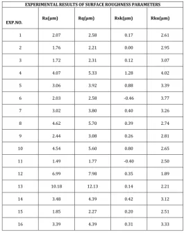
Table -3:The Measurement of Surface Roughness:

EXPERIMENTAL RESULTS OF SURFACE ROUGHNESS PARAMETERS

EXP.NO. Ra(µm) Rq(µm) Rsk(µm) Rku(µm)

1 2.07 2.58 0.17 2.61

2 1.76 2.21 0.00 2.95

3 1.72 2.31 0.12 3.07

4 4.07 5.33 1.28 4.02

5 3.06 3.92 0.88 3.39

6 2.03 2.58 -0.46 3.77

7 3.02 3.80 0.40 3.26

8 4.62 5.70 0.39 2.74

9 2.44 3.08 0.26 2.81

10 4.54 5.60 0.80 2.65

11 1.49 1.77 -0.40 2.50

12 6.99 7.98 0.35 1.89

13 10.18 12.13 0.14 2.21

14 3.48 4.39 0.42 3.12

15 1.85 2.27 0.20 2.51

16 3.39 4.39 0.31 3.33

3. Optimization of Turning Process

3.1 Evaluation of optimal process condition:-

In GRA, Experimental data of expected output feature of quality characteristic is first normalised, ranging from zero to one, called Grey Relational Generation.

The normalised data corresponding to both the criteria are calculate as

(a)When the smaller-the-better is a characteristic of the original sequence, then the original sequence should be normalized as follows:

Xi (k) = max Yi (k) – Yi (k)/max Yi (k) – min Yi (k) (b)For the larger-the-better characteristic of the original sequence can be normalized as follows:

Xi (k) = Yi (k) – min Yi (k)/max Yi (k) – min Yi (k) where Xi(k) is the value after the grey relational

generation, min Yi(k) is the smallest value of Yi(k) for the kth

response and max Yi(k) is the largest value of Yi (k) for the kth

response. An ideal sequence is [X0(k) (k=1,2,3,....n)] for the

responses.

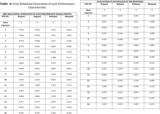
Table -4: Shows parametric optimization was done for turning process by using the following criterion for smaller-the-better concept of all roughness parameters.

Stainless Steel 304

Chemical composition (%)

C Mn Si P S Cr

0.08 2 0.75 0.045 0.03 20

Mechanical

properties Tensile Strength(Mpa) Yield Strength (MPa)

Elongation Hardness

[image:2.595.52.279.185.268.2] [image:2.595.44.286.329.507.2]

(3)

[image:3.595.39.565.122.495.2]

Xi (k) = max Yi (k) – Yi (k)/max Yi (k) – min Yi (k)

Table -4: Grey Relational Generation of each Performance Characteristic

GREY RELATIONAL GENERATION OF EACH PERFORMANCE CHARACTERISTIC

Ideal sequence

1 1 1 1

1 0.933 0.922 1.354 0.662

2 0.969 0.958 1.561 0.502

3 0.974 0.948 1.415 0.446

4 0.703 0.656 0.000 0.000

5 0.819 0.792 0.488 0.296

6 0.938 0.922 -1.000 0.117

7 0.824 0.804 1.073 0.357

8 0.640 0.621 1.085 0.601

9 0.891 0.874 1.244 0.568

10 0.649 0.630 0.585 0.643

11 1.000 1.000 -1.073 0.714

12 0.367 0.401 1.134 1.000

13 0.000 0.000 1.390 0.850

14 0.771 0.747 1.049 0.423

15 0.959 0.952 1.317 0.709

16 0.781 0.747 1.183 0.324

The definition of Grey Relational Grade in the course of Grey Relational Analysis is to reveal the degree of relation between the n sequences [X0(k) and Xi(k), i=1,2,3,....n]. The

Grey Relational Coefficient ξi(k) can be calculated

ξi (k) = [Δmin + Ψ Δmax] / [Δ0i (k) + Ψ Δmax]

where Δoi (k) is the deviation sequence of the reference

sequence and comparability sequence

Δ0i (k) = || Xo (k) – Xi (k) || “Ψ” is the distinguishing coefficient and 0≤Ψ≤1

Table -5: Evaluation of Δ0i for each of the responses

EVALUATION OF Δ0I FOR EACH OF THE RESPONSES

Ideal sequence

1 1 1 1

1 0.067 0.078 0.354 0.338

2 0.031 0.042 0.561 0.498

3 0.026 0.052 0.415 0.554

4 0.297 0.344 1.000 1.000

5 0.181 0.208 0.512 0.704

6 0.062 0.078 0.000 0.883

7 0.176 0.196 0.073 0.643

8 0.360 0.379 0.085 0.399

9 0.109 0.126 0.244 0.432

10 0.351 0.370 0.415 0.357

11 0.000 0.000 0.073 0.286

12 0.633 0.599 0.134 0.000

13 1.000 1.000 0.390 0.150

14 0.229 0.253 0.049 0.577

15 0.041 0.048 0.317 0.291

16 0.219 0.253 0.183 0.676

Considereing Δ0i value from table.4 and distinguishing

coefficient,Ψ where 0≤Ψ≤1, the grey relational coefficients ξi(k) are calculated by using the following relationship

ξi (k) = [Δmin + Ψ Δmax] / [Δ0i (k) + Ψ Δmax]

where Δmin is the smallest value of Δ0i, Δmax is the largest value

of Δi of the corresponding parameters and ‘Ψ’, the

(4)

Table -6: Evaluation of Δ0i for each of the responses

GREY RELATIONAL COEFFICIENTS WITH ΨRa = ΨRq = ΨRsk = ΨRku = 0.2 FOR EACH PERFORMANCE CHARACTERISTIC

Ideal

sequence 1 1 1 1

1 0.749 0.719 0.361 0.372

2 0.866 0.826 0.263 0.287

3 0.885 0.794 0.325 0.265

4 0.402 0.368 0.167 0.167

5 0.525 0.490 0.281 0.221

6 0.763 0.719 1.000 0.185

7 0.532 0.505 0.733 0.237

8 0.357 0.345 0.702 0.334

9 0.647 0.613 0.450 0.316

10 0.363 0.351 0.325 0.359

11 1.000 1.000 0.733 0.412

12 0.240 0.250 0.599 1.000

13 0.167 0.167 0.339 0.571

14 0.466 0.442 0.803 0.257

15 0.830 0.806 0.387 0.407

16 0.477 0.442 0.522 0.228

After averaging the Grey Relational Coefficients, the Grey Relational Grade γi can be computed as

γ i = 1/n

where

γ i represents GRG

n is the number of process responses

The higher value of grey relational grade corresponds to intense relational degree between the reference sequence X0(k) and the given sequence Xi(k). the reference sequence

X0(k) represents the best process sequence, therefore,, higher

grey relational grade means that the corresponding parameter combination is closer to the optimal.

Table -7: Overall Grey Relational Grade

OVERALL GREY RELATIONAL GRADE

EXP.NO. _{RELATIONAL GRADE}OVERALL GREY RANK

1 0.550 6

2 0.560 5

3 0.567 4

4 0.276 16

5 0.379 13

6 0.667 2

7 0.502 9

8 0.435 11

9 0.507 8

10 0.350 14

11 0.786 1

12 0.522 7

13 0.311 15

14 0.492 10

15 0.608 3

16 0.417 12

Table -8: Shows the S/N ratio based on the larger-the-better criterion for overall grey relational grade calculated by using

S/N= -10 Log[1/n 1/yi2 ]

S/N RATIO FOR OVERALL GREY RELATIONAL GRADE

EXP. NO. S/N RATIO

1 -5.192

2 -5.036

3 -4.928

4 -11.182

5 -8.427

6 -3.517

7 -5.986

8 -7.230

9 -5.900

10 -9.119

11 -2.092

12 -5.647

13 -10.145

14 -6.161

15 -4.322

(5)

4. Result and Discussion:

The main objective of the experiment is to optimize the turning parameters (Speed, Feed, Depth of cut, Type of Tool) The experimental data for the surface roughness values and the calculated signal-to-noise ratio are shown in Table 8, for Stainless Steel. The S/N ratio values of the surface roughness are calculated, using the larger-the-better characteristics.

Table 8, shows the surface roughness along with its computed S/N ratio value. Average S/N ratio for each level of experiment is calculated based on the value of Table 3.

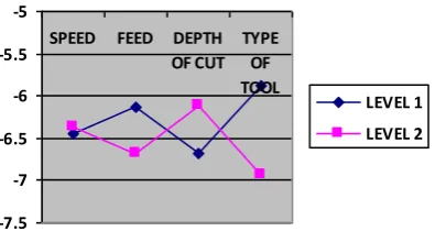
Based on the calculated S/N ratio values, it can be seen that a speed of 485 rpm and a feed rate of 0.025 mm/rev and Depth of cut of 0.9mm with High Carbon steel tool gives the optimum values for turning of Stainless steel.

-7.5 -7 -6.5 -6 -5.5 -5

SPEED FEED DEPTH OF CUT

TYPE OF TOOL

[image:5.595.67.265.320.425.2]

LEVEL 1 LEVEL 2

Fig -3: Parameters Vs Avg. S/N Ratio

[image:5.595.72.241.532.602.2]

fig – 3:gives an Interaction effects plot for cutting parameters vs Avg. S/N ratio to determine the optimum surface roughness value.

Table -9: Optimum values of factors and their levels

Parameters Optimum

Value

Speed, rpm 485

Feed, mm/rev 0.025

Depth of Cut, mm 0.9

Type of Tool High Carbon

Steel

5. CONCLUSIONS

The present investigation aimed at optimization of surface roughness during turning of Stainless Steel work piece. This analysis was carried out by developing surface roughness models of Ra, Rq, Rsk, Rku based on full factorial in

Taguchi optimization technique. Main effect plots were drawn manually & also using Taguchi design & compared with each other.

Surface roughness & the cutting parameters have highly non-linier relationships among them. The minimal surface roughness is obtained at a combination of speed (485 rpm), feed (0.025 mm/rev), and depth of cut (0.9mm), type of tool (High Carbon Steel).

Experiment no. 11 is obtained as the optimal solution by Grey relational based Taguchi method of optimization. The experiment, when stainless steel is turned with 485rpm speed, 0.025mm/rev feed having 0.9mm depth of cut with high Carbon steel tool is the obtained optimal solution. The same experiment no. 11 is decided as optimal from S/N ratio analysis also.

The predicted values and calculated values are very close to each other, which indicate the Accuracy of the developed model

REFERENCES

[1] Wu, H.H., “The introduction of Grey Analysis”, Gauli

Publishing Co., Taipei, 1996.

[2] Knowles, Peter Reginald (1987), Design of structural

steelwork (2nd ed.), Taylor & Francis, p. 1, ISBN 978-0-903384-59-9

[3] Ziliang.W, and Sifeng.L. Extension of Grey Superiority

Analysis, Liu S.F. et al. Grey system Theory and its application, Science Press, Beijing, China,2004).

[4] Kun-lin Wen, The grey system analysis and its

application in gas breakdown and var compensator finding(invited paper), Int. Journal of computational Cognition 2(1)(2004) 21-44.)

[5] K.C Chang and M-F, Yeh, Grey-relational analysis based

approach for data clustering, IEEE Proc,_Vis. Image Signal Process., Vol.152,No,2, April 2005, pp165-172.

[6] Lu, H.C., Yeh,M-F.: Robot path planning based on

modified grey analysis, Cybern. Syst., 2002, 33,(2), pp 129-159.

[7] R. Nicole, “Title of paper with only first word

capitalized,” J. Name Stand. Abbrev., in press.

(6)

BIOGRAPHIES

T.Naga Sushma

PGStudent,

Department of Mechanical Engg., DMS SVH College of Engineering, Machilipatnam,

Andhra Pradesh, India.

Smt. P.S.Naga Sree Assistant Professor

Department of Mechanical Engg., DMS SVH College of Engineering, Machilipatnam,

Dr. Doradla Raja Ramesh Professor & H.O.D,

Department of Mechanical Engg., SVIET, Nandamuru,

Sri.T.Ravi kumar

Associate Professor & H.O.D, Department of Mechanical Engg., DMS SVH College of Engineering, Machilipatnam,

Implementation of Taguchi Technique for Optimization of Performance Parameters of Turning Process