Automatic Generation Control of an Interconnected Power System Before and After Deregulation

(1)

Automatic Generation Control of an Interconnected

Power System Before and After Deregulation

Pardeep Nain

Assistant Professor UIT, Hansi Haryana, India

K. P. Singh Parmar

Assistant Director (Technical) CAMPS, NPTI, Faridabad

Haryana, India, 121003

A. K. Singh

Associate Professor DCRUST, Murthal

Haryana, India

ABSTRACT

This paper presents the particle swarm optimization (PSO)

technique to optimize the integral controller gains for the automatic generation control (AGC) of the interconnected power system before and after deregulation. Each control area includes the dynamics of thermal systems. The AGC in conventional power system is studied by giving step load perturbation (SLP) in either area. The AGC in deregulated environment is studied for three different contract scenarios. To simulate bilateral contracts in deregulated system, the concept of DISCO participation matrix (DPM) is applied.

Keywords:

Automatic generation control, bilateral contract, deregulation; integral controller, particle swarm optimization

1. INTRODUCTION

In the power system, numbers of utilities are interconnected through a tie-line by which power is exchanged between them [1]-[3]. Any sudden load perturbation in power system can cause variation in tie-line power interchange and frequency. AGC is used in the power system to keep frequency of control areas at its nominal value and tie-line power exchange for different control areas at their scheduled values [4]-[7]. In conventional power system, utilities have their own generation, transmission and distribution. Deregulated environment can consist of a system operator (SO), distribution companies (DISCOs), generation companies (GENCOs), and transmission companies (TRANSCOs). There is some difference between the AGC operation in conventional and deregulation environment. After deregulation, simulation, optimization and operation are changed but their basic idea for AGC is keep same [8]-[9]. In the new environment, DISCOs may contract power from any GENCOs and SO have to supervise these contracts. DISCO participation matrix (DPM) concept is taken to understand the several contracts that are implemented by the GENCOs and DISCOs [10].

Classical approach considers integral square error (ISE) for optimization of integral controller gain [11], [12]. This is a time consuming and trial and error method. Different numbers of approaches such as optimal, classical, artificial neural network (ANN), fuzzy logic and genetic algorithm (GA) have been used for optimization of controller parameters [13]-[15]. Many authors [16], [17] tried to use genetic algorithm (GA) for designing of controller more efficiently than the controller based on classical approach. Recently authors have found some drawbacks in GA algorithm [18]. At the other side, the premature convergences of GA degrade its searching ability.

characteristics. Compared to other optimization techniques, PSO is a more faster, robust and easy to use. PSO have been used in different areas: fuzzy system control, artificial neural network training, function optimization, and several areas where GA is used.

2. OPTIMIZATION

TECHNIQUE

PSO is one of the most used and well known optimization techniques. Introduced by Dr. Eberhart and Dr. Kennedy [20] in 1995, PSO defines a population based optimization algorithm. In PSO, each particle is initialized by giving them random number.

The cost function which to be minimized is given by:

J = )2 + ( )2 + ( )2}dt (1)

Where T is the simulation time.

Let represent the particle’s position and u represent the flight

velocity in a search space. Hence, the location of each kth particle is denoted as =( , ,…, ) in the

-dimensional space. The previous best position of the kth particle is stored and given as =( , ,…….. ). The best particle among all these particles is taken as global best particle, given by . The velocity for the kth particle is

denoted as = ( , , ……..., ).

The updated position and velocity of all particles may be determined by using the distance and the current velocity from

to as given in the following equations [20].

= * i + *r1( )*( - ) + *r2( )*(

)

(2)

= + (3)

In the above equation (2), i is known as the inertia weight factor and and are known as the acceleration coefficients that attract all particles towards the and positions. r1( ) and r2( ) are the uniform random numbers must taken

between [0,1]. The term r1 ( )*( - ) is called the

cognitive component. The term r2 ( )*( - ) is called the

social component. Low values of acceleration coefficients result in wandering of particle away from the target region. In the other side, a high values of same result in sudden movement of particle towards or past the target region. Acceleration coefficients and are mostly taken as 2 according to pervious experiences [20].

(2)

requires lesser iterations. In general, the inertia weight i can be represented as [20],

i= –[( – )* ]/( ) (4)

Here the maximum value of inertia weight is represented by

, the minimum value of inertia weight is represented by , number of current iterations are represented by and

number of maximum iterations are represented by .

3. SYSTEM INVESTIGATED

3.1 Two- area interconnected conventional

power system

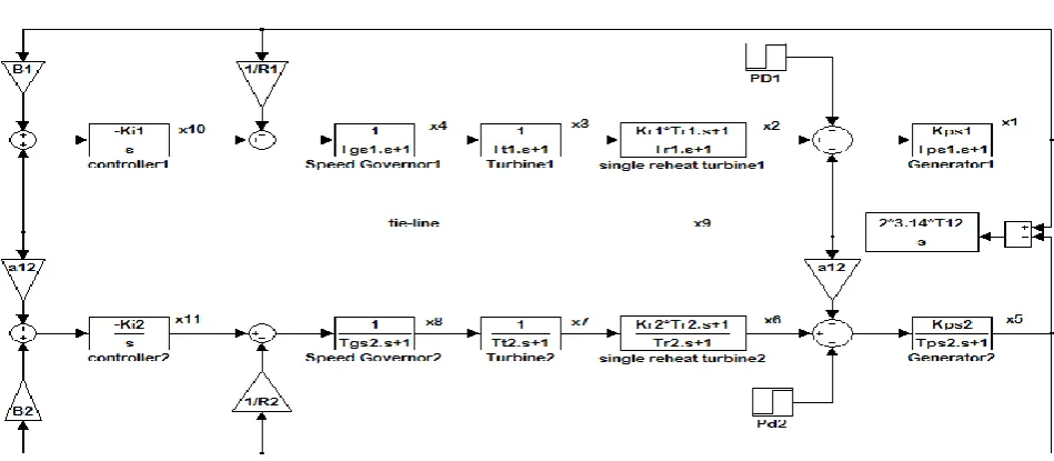
The AGC of a two-area interconnected power system is presented in this section. The simulation model presented is based on the concepts described in [4]-[7]. In [1]-[4] the system parameters are shown. Each control area is identical and consists of thermal system with reheat turbine. MATLAB version 7.10 is used to obtain dynamic response of ∆f1, ∆f2, and ∆Ptie-line1-2 for 1% SLP in either area. MATLAB simulation model of a conventional two-area system is represented in Fig. 2.

3.3.1 Simulation, results and discussion

In this case, integral controller gains (KI1 & KI2) are optimized by minimizing the cost function (J) using PSO technique. 1% SLP is given in area 1. The optimum values of integral gains found are KI1 = 0.275 and KI2 = 0.394. The frequency deviation response of area 1 and area 2 are shown in Fig. 4 (a) and (b) respectively and tie-line power response is shown in Fig. 4 (c). The frequency and tie line power deviations settle to zero. Further, it is observed that dynamic responses thus obtained satisfy the requirement of AGC problem in terms of settling time and steady state error.

[image:2.595.76.295.616.686.2]

3.2 AGC of two-area interconnected

power system in deregulated environment

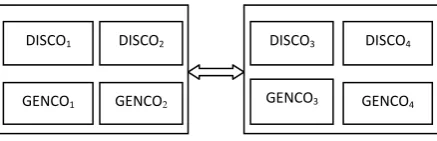
Deregulated system contains various GENCOs and DISCOs, a DISCO has a freedom to make contract with GENCOs in another control area independently [10]. Hence it is known “bilateral transaction”. All these transactions can be supervised through a SO. SO has an impartial entity and controls a lot of ancillary services and AGC is one of them. In restructured environment, DISCOs have a liberty to demand the power from various GENCOs. To understand the visualization of contract easier, the concept of DPM is used. In DPM, the number of the columns equals to the number of DISCOs and the number of the rows equals to the number of GENCOs in the system. Each element of this matrix is a fraction of total load contracted by a DISCO toward a GENCO. The total sum of all the elements of a column in the DPM is equal to unity [8]-[10].

Fig. 1. The configuration of two-area interconnected power system in restructured environment.

DPM =

11 12 13 14

21 22 23 24

31 32 33 34

41 42 43 44

cpf





































(5)

Where

cpf

represents “contract participation factor”. It is

noted that

1

ij i

cpf





. In restructured environment, change in the load demand of a DISCO results in change of a local load in the same DISCO area. This corresponds to the local load power system block. The coefficient, which give this sharing, are represented as “area control error (ACE) participation factors” (

apf

) and

1

n

j j

apf





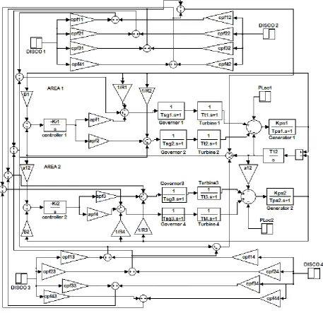
where n is the number of GENCOs in the each control area. Unlike traditional AGC system, any DISCO can demand for the power supply from any GENCO.

The model presented by Donde et. al [10] is considered in this case for further study and analysis of AGC using MATLAB simulation and design of controllers based on PSO optimization. There are two DISCOs and two GENCOs in each control area as shown in Fig. 1. GENCOs are thermal units. The MATLAB simulation model of two-area thermal system in deregulated environment is shown in Fig. 3.

The scheduled tie-line power flow at steady state in case of two-area power system flow is represented as follow [10]:

∆Ptie-line1-2, schd = [power supplied from GENCOs of area 1to DISCOs of area 2] - [power supplied from GENCOs of area 2 to

DISCOs of area 1]. (6)

The tie-line power error may be represented as follows [10]:

1 2, 1 2, 1 2,

tie line error tie line actual tie line schd

P

_ _

P

_ _

P

_ _



 



(7)

ACE signal for two-area as follow:

1 1 1 tie line1 2,error

ACE

   

B f

P

_ _ (8)

2 2 2 12 tie line1 2,error

ACE

  

B

f

a



P

_ _ (9)

a12 is the ratio of rated power of area I and area II and a12 = -1. The closed loop two area power system in Fig. 3 is characterized in the steady state form as follows:

cl cl

x

A x

B u







(10) Where

x

is the state vector and

u

is the vector of demand of

the DISCOs.

A

cl and

B

clmatrices are constructed from Fig. 3. In this paper, as in [10], three different cases are studied. GENCO2

DISCO1

GENCO1

DISCO2

GENCO3 GENCO4

(3)

Case 1:

In base case, all of them

apfs

are same as 0.5 for all the GENCOs. DPM is formed by only taking cpf11, cpf12, cpf21, cpf22 are equal to 0.5 as in [10].

DPM =

0.5

0

0.5

0

0 























₍₁₁₎

In the steady state, the GENCO’s generation can equal to the contract demand of the DISCOs with it, given as follow:

Gi ij Lj

i

P

cpf

P









(12)

Where ∆ is the total demand of DISCOj. In this case, DISCOs belongs to other area do not contract the GENCOs belongs to area 2 and as a result are zero change in generation power take place in steady state.

Case 2:

In this case, DISCOs can contract with the GENCOs in its own and other area for power as per the following DPM:

DPM =

0.5 0.25 0

0.3

0.2 0.25 0

0

0 0.25 1

0.7 0.3 0.25 0

0 























₍₁₃₎

This is consider that DISCOs demands 0.1 pu MW total power from GENCOs as denoted by elements in DPM and all GENCOs participated in AGC as represented by the following

apfs

;

apf

₁=

0.75,

apf

₂= 0.25,

3

apf

= 0.25,

apf

₄ = 0.5. The scheduled power on the tie-line is given as follow [10]:

2 4 4 2

1 2,

1 3 3 1

tie line schd ij Lj ij Lj

i j i j

P

_ _

cpf

P

cpf

P

   







 





(14) Case 3:

It may happen that when a DISCO demands more power than the contracted power, the contract violates. It is to be noted that this un-contracted power demands have to be met by the GENCOs of the same area as the DISCO [10]. The more power can be considered as a local load. Case 2 considers again with addition that DISCO1 demands 0.1 pu MW more [10].

In area 1 total local load = DISCO1 load+ DISCO2 load = (0.1 + 0.1) + 0.1 = 0.3 pu MW

Similarly, In area 1 total local load = DISCO3 load + DISCO4 load

= 0.1 + 0.1 = 0.2 pu MW

The un-contracted load of DISCO1 is reflected by GENCOs in its area.

3.2.1 Simulation, results and discussion

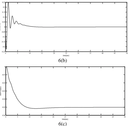
In this section, integral controller gains of each control area in the two-area power system in deregulated environment are optimized using PSO technique. The power system simulation is done using MATLAB. The cost function J obtained using equation (1) is optimized by the PSO technique. In case 1, the optimum values of integral gains are KI1 = 1 and KI2 = 0.1556. The dynamic responses of frequency and tie-line power are shown in Fig. 5 (a)-(c). In case 2, the two optimum values of integral gains are KI1 = 0.0377 and KI2 = 0.6032. The dynamic responses of frequency and tie-line power are shown in Fig. 6 (a)-(c). In case 3, the two optimum values of integral gains are KI1 = 1.5 and KI2 = 0.9069. The dynamic responses of frequency and tie-line power are shown in Fig. 7 (a)-(c).

[image:3.595.62.537.515.722.2]

(4)

[image:4.595.71.529.75.518.2]

Fig. 3.MATLAB simulation model of two-area thermal system in deregulated environment

4(a) 4(b)

0 5 10 15 20 25 30 35 40 45 50 -0.03

-0.025 -0.02 -0.015 -0.01 -0.005 0 0.005

time(sec)

d

e

lf

1

(H

z

)

0 5 10 15 20 25 30 35 40 45 50 -0.03

-0.025 -0.02 -0.015 -0.01 -0.005 0 0.005

time(sec)

d

e

lf

2

(H

(5)

4(c)

Fig. 4 (a) Frequency response of area 1. (b) Frequency response of area 2. (c) Deviation of tie-line power.

5(a)

5(b)

5(c)

6(a)

6(b)

6(c)

7(a)

7(b)

7(c)

0 5 10 15 20 25 30 35 40 45 50 -8 -7 -6 -5 -4 -3 -2 -1 0 1x 10

-3 time(sec) d e lP 1 2 (p u M W )

0 5 10 15 20 25 30 35 40 45 50 -0.25 -0.2 -0.15 -0.1 -0.05 0 0.05 0.1 0.15 0.2 0.25 time(sec) d e lf 1 (H z)

0 5 10 15 20 25 30 35 40 45 50 -0.02 -0.015 -0.01 -0.005 0 0.005 0.01 0.015 time(sec) d e lf 2 (H z)

0 5 10 15 20 25 30 35 40 45 50 -10 -8 -6 -4 -2 0 2 4x 10

-3 time(sec) d e lP 1 2 (p u )

0 5 10 15 20 25 30 35 40 45 50 -0.3 -0.25 -0.2 -0.15 -0.1 -0.05 0 0.05 0.1 time(sec) d e lf 1 (H z)

0 5 10 15 20 25 30 35 40 45 50 -0.25 -0.2 -0.15 -0.1 -0.05 0 0.05 0.1 0.15 0.2 0.25 time(sec) d e lf 2 (H z)

0 5 10 15 20 25 30 35 40 45 50 -0.06 -0.05 -0.04 -0.03 -0.02 -0.01 0 time(sec) d e lP 1 2 (p u )

0 10 20 30 40 50 60 70 80 90 100 -0.5 -0.4 -0.3 -0.2 -0.1 0 0.1 0.2 time(sec) d e lf 1 (H z)

0 10 20 30 40 50 60 70 80 90 100 -0.4 -0.3 -0.2 -0.1 0 0.1 0.2 0.3 time(sec) d e lf 2 (H z)

0 10 20 30 40 50 60 70 80 90 100

[image:5.595.77.533.79.720.2] [image:5.595.67.284.84.632.2] [image:5.595.315.538.91.309.2] [image:5.595.310.542.331.697.2]

(6)

4. CONCLUSION

In this paper, AGC of an interconnected power system before and after deregulation is presented. PSO technique is applied to optimize the controller gains. In the conventional power system the frequency and tie-line power deviation responses are obtained for 1% SLP. It is found that frequency and tie line power deviation responses settle with zero steady state error and satisfy the AGC requirements.

In deregulated environment, bilateral contracts between DISCOs in one control area and GENCOs in another control area are considered. Bilateral contracts make the base for choosing the elements of DPM. The AGC is studied for different possible contracts in deregulated environment. The tie-line scheduled power flow between two controls areas matches with the contract. The dynamic responses obtained for different possible contracts satisfy the AGC requirements.

5. REFERENCES

[1] C. Concordia and L. K. Kirchmayer, “Tie-line power frequency control of electric power system: Part II,” AISE Trans, III-A, vol. 73, pp. 133–146, Apr. 1954.

[2] O. I. Elgerd and C. E. Fosha, “Optimum megawatt-frequency control of multiarea electric energy systems,” IEEE Trans. Power App. Syst., vol. PAS-89, no. 4, pp. 556–563, Apr. 1970.

[3] C. E. Fosha and O. I. Elgerd , “The megawatt-frequency control problem-A new approach via optimal control theory,” IEEE Trans. Power App. Syst., vol. PAS-89, no. 4, pp. 563–577, Apr. 1970.

[4] D. P. Kothari and I. J. Nagrath, “Power System Engineering”, 2nd edition, TMH, New Delhi, 2010.

[5] O. I. Elgerd , “Electric Energy Systems Theory an Introduction,” 2nded. New Delhi, India: Tata McGraw-Hill, 1983, pp. 299–33.

[6] P. Kundur, “Power system stability & control.” New York: McGraw-Hill, 1994, pp. 418-448.

[7] Nanda J, Mangla A, Suri Sanjay, “Some new findings on automatic generation control of an interconnected hydrothermal system with conventional controllers.” IEEE Trans Energy Convers 2006;21(1):187–94.

[8] Bhatt Praghnesh, Roy Ranjit, Ghoshal SP. “Optimized multi area AGC simulation in restructured power systems.” Int J Electric Power Energy Syst 2010;32(4):311–22.

[9] Christie RD, Bose A. “Load frequency control issues in power system operations after deregulation.” IEEE Trans Power System 1996;11(3):1191–200.

[10] Donde V, Pai MA, Hiskens IA. Simulation and optimization in an AGC system after deregulation. IEEE Trans Power Syst 2001;16(3):481–9.

[11] M. L. Kothari, P. S. Satsangi and J. Nanda, “Sampled data automatic generation control of interconnected reheat thermal systems considering generation rate constraints,” IEEE Trans. on Power Apparatus and systems,vol.PAS-100, no.5, pp 2334-2342, May1981.

[12] L. Hari, M. L. Kothari and J. Nanda, “Optimum selection of speed regulation parameters for automatic generation control in discrete mode generation rate constraints,” IEE Proc. C, vol.138, no.5, pp 401-406, Sep 1991.

[13] Demiroren A, Zeynelgil HL, “GA application to optimization of agc in three-area power system after deregulation.” Int J Electr Power Energy Syst 2007;29:230– 40.

[14] G. A. Chown, R. C. Hartman, “Design & Experience of Fuzzy Logic Controller for Automatic Generation Control (AGC),” IEEE Trans. Power Systems, vol. 13, No. 3, pp. 965-970, Aug. 1998.

[15] F. Beaufays, Y. Abdel-Magid and B. Widrow, “Application of neural network to load frequency control in power systems,” Neural Networks vol.7, no.1, 183-194,1994.

[16] S. P. Ghoshal and S. K. Goswami, “Application of GA based optimal integral gains in fuzzy based active power-frequency control of non-reheat and reheat thermal generating systems,” Elect. Power Syst. Res., vol. 67, pp. 79–88, 2003.

[17] S. P. Ghoshal, “Application of GA/GA-SA based fuzzy automatic generation control of a multi-area thermal generating system,” Elect. Power Syst. Res., vol. 70, pp. 115–127, 2004.

[18] R. C. Eberhart and Y. Shi, “Comparison between genetic algorithms and particle swarm optimization”, Proceedings of IEEE Int. Conf. on Evol. Comput., pp. 611-616, 1998.

[19] M. A. Abido, ‘‘Optimal design of power-system stabilizers using particle swarm optimization,’’ IEEE Trans. Energy Conversion., vol. 17, no. 3, pp. 406-413, Sep. 2002.

[20] D. P. Kothari and J. S. Dhillon, “Power System Optimization”, 2nd