A Two Phase Algorithm for Fuzzy Time Series
Forecasting using Genetic Algorithm and Particle Swarm
Optimization Techniques
Usman Amjad
Department of Computer Science, University of Karachi
Tahseen A. Jilani
Department of Computer Science,University of Karachi
Farah Yasmeen
Department of Statistics,University of Karachi
ABSTRACT
Fuzzy Time series is being used for forecasting since last two decades for forecasting. Nature inspired computing techniques like other domains are now being used for optimization purpose in Fuzzy Time Series forecasting models to get improved results. In this paper we have presented a new algorithm for multivariate fuzzy time series forecasting having two phases. Genetic Algorithm and Particle Swarm Optimization techniques are used in this algorithm for optimization. We applied our algorithm on Taiwan forex Exchange (TAIFEX) index and got better results and minimized error rate as compared to previous methods.
General Terms
Nature inspired computing; Time Series forecasting
Keywords
Fuzzy time series; two-factor high-order fuzzy logical relationships; Genetic Algorithm, Particle Swarm Optimization; TAIFEX index.
1.
INTRODUCTION
Forecasting is prediction of unseen values of some sequence. It holds significance in economic and financial modeling as entrepreneurs use predicted values for business planning and taking key decisions. In the last two decades Fuzzy Time Series (FTS) is being used for forecasting purpose. Song and Chissom [1, 2] used the concept of FTS and forecasted number of enrollments of the University of Alabama. Many other researchers proposed their models for enrollments forecasting of the University of Alabama ([3], [4], [5], [6], [7], [8], [9], [10] and [11]), temperature prediction [12, 13] and car road accidents [14, 15] using fuzzy time series. Huarng [7] presented heuristic based model for fuzzy time series forecasting. Jilani and Burney [14] presented M-factor high order fuzzy time series forecasting model for car road accident data. Jilani and Burney [16] presented new heuristic based approach for frequency density based partitioning for fuzzy time series forecasting of stock market.
In the recent years many researchers started applying Nature inspired computation (NIC) techniques for optimization purpose in FTS forecasting. Kuo et al. [17] and Huang et al.[18] proposed Particle Swarm Optimization (PSO) based FTS forecasting models for enrollments data of the University of Alabama. Park et al. [19] proposed a forecasting model for TAIFEX and KOSPI-200 index, which was based on FTS and swarm intelligence. Jilani et. al. [20] proposed a PSO based FTS forecasting model for car road accidents. Jilani et. al. presented a hybrid algorithm based on Genetic Algorithm (GA) and PSO for forecasting TAIFEX
and KSE-100 index. Jilani et. al. [22] presented a trend based heuristic approach using GA for forecasting car road accidents.
In this paper we have applied genetic algorithm in first phase to optimize weights, and in second phase we used those weights and optimized interval length to get best forecasting result.
2.
Few Basic Concepts of Fuzzy Time
Series
To deal with the ambiguity and uncertainty of real world problems, the concept of fuzzy logic and fuzzy set theory (Zadeh [23]) was introduced. Thus a time series is introduced with fuzziness termed as fuzzy time series (Song and Chissom [24]) introduced the concept of fuzzy time series and since then a number of variants were published by many authors. Some of the essentials are being reproduced to make the study self-contained.
Definition 1: Let Y(t), (t = …,0,1, 2,…) be the universe of discourse and Y(t)
Y
(
t
)
R
. Assume that f(ti), i = 1, 2, . . ., is defined in the universe of discourse Y(t) and F(t) is a collection of f(ti), (t = ..., 0,1,2, ...), then F(t) is called a fuzzy time series of Y(t), i = 1,2,3,.... Using fuzzy relation, we define F(t) = F(t −1) o R(t, t −1) where R(t, t −1) is a fuzzy relation and “o” is the max–min composition operator, then F(t) is caused by F(t − 1) where F(t) and F(t −1) are fuzzy sets.Definition 2: Let F(t) be a fuzzy time series and let R(t,t-1) be a first-order model of F(t). If R(t,t-1) = R(t-1,t-2) for any time t, then F(t)is called a time-invariant fuzzy time series. If R(t,t-1) is dependent on time t, that is, R(t,t-R(t,t-1) may be different from R(t-1,t-2) for any t, then F(t) is called a time-variant fuzzy time series.
Definition 3: Let F(t) be a fuzzy time series. If F(t) is caused by F(t−1), F(t−2),…,F(t−n), then the nth-order fuzzy logical relationship is represented by F(t−n) ,…, F(t−2), F(t−1)→F(t) where F(t−1), F(t−2) , …, F(t−n) and F(t) are all fuzzy sets, where F(t−1) ,F(t−2) ,…, F(t−n) is called the antecedent and F(t) is called the consequent of the nth-order fuzzy logical relationship.
3.
An overview of Genetic Algorithm
selection, crossover and mutation are applied to get offspring. Same operators are repeatedly applied until stopping criteria is not met.
Selection refers to the procedure of selecting chromosomes from the population for offspring production. Usually the chromosomes with good fitness value are selected. Many schemes exist for selection of chromosomes including roulette wheel and tournament selection.
Crossover refers to the procedure of recombination of multiple chromosomes to produce offspring. Selected chromosomes exchange information with each other using crossover operator by swapping genes after the crossover point. Crossover point is found randomly by the length of chromosomes i.e. number of genes in a chromosome.
Mutation refers to phenomenon of introduction of a new property in offspring by changing gene values. It is very rare in offspring but when it occurs, it puts a great impact on fitness of chromosome. Mutation point is found randomly in range of chromosome length and the gene at that point is replaced by some other value.
4.
Particle Swarm Optimization
Particle Swarm Optimization is a computational method that optimizes a problem by iteratively trying to improve a candidate solution with regard to a given measure of quality [27]. PSO optimizes a problem by having a population of candidate solutions, here dubbed particles, and moving these particles around in the search space according to simple mathematical formulae over the particles position and it is also guided toward the best known position in the search space, which are updated as better positions are found by other particles.
In other words we can say that the core concept of PSO lies in accelerating each particle toward its pbest which was achieved so far by that particle, and the gbest which is the best value obtained so far by any particle in the neighborhood of that particle, with a random weighted acceleration at each time step. A particle’s velocity and position are updated as follows.
( 1) ( ) ( ) ( ) ( )
1 1
(
)
2 2(
)
t t t t t
i i i i
v
w
v
c r
pbest x
c
r
gbest x
(1)
(t 1) ( )t (t 1)
X
X
v
(2)Where X and V are position and velocity of particle respectively, w is inertia weight, c1 and c2 are positive constants, called acceleration coefficients which control the influence of pbest and gbest on the search process, P is the number of particles in the swarm, r1 and r2 are random values in range [0, 1].
PSO has some drawbacks, such as when the search space is high its convergence speed becomes very slow near global optimum. Another drawback is its nature to a fast and premature convergence in mid optimum points.
The Basic Algorithm for PSO is as under:
1.Create a ‘population’ of particles uniformly distributed over X.
2.Initialize every particle.
3.Calculate fitness value for each particle.
4.If current fitness value of a particle is better than the personal best (pbest) of particle set this as pbest. 5.Choose the particle with the best fitness value of all
particles as the global best (gbest).
6.Update particles velocities according to equation 1. 7.Move particles to their new positions according to
equation 2.
8.Go to step 2 until stopping criteria are satisfied.
5.
Two phase forecasting model based on
GA and PSO
In this section, a new fuzzy time series forecasting model will be presented based on GA and PSO. The proposed technique
will be applied on
[image:2.595.314.533.348.658.2]TAIFEX index for the period of 3rd August 1998 to 30th September 1998. Our main factor in proposed method is actual TAIFEX (X) and secondary factor the TAIEX index (Y).
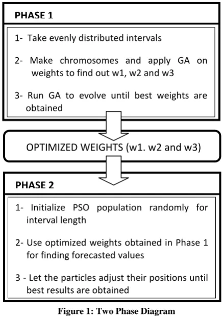
Figure 1: Two Phase Diagram
5.1
Phase 1
In the first phase we have applied GA to optimize weights w1, w2, w3 used in formula (Jilani, Burney [15]).
Step 1: Define and Partition the universe of discourse U of the main-factor into n intervals u1, u2,…,un, where u1 = [Dmin−D1, x1), u2 =[x1, x2),…, un =[xn−1, Dmax+D2] and
PHASE 1
1- Take evenly distributed intervals
2- Make chromosomes and apply GA on weights to find out w1, w2 and w3
3- Run GA to evolve until best weights are obtained
OPTIMIZED WEIGHTS w1. W2 and w3
OPTIMIZED WEIGHTS (w1. w2 and w3)
PHASE 2
1- Initialize PSO population randomly for interval length
2- Use optimized weights obtained in Phase 1 for finding forecasted values
1 -n 2
1
x
x
x
. Similarly partition the universe of discourse of secondary factor into m intervals v1, v2,…,vm, where
v1 = [y1, Emax+E2], v2 = [y2, y1),…,vm =[Emin−E1, ym−1)
, and
y
1
y
2
....
y
m1. In the proposed algorithm we partitioned universe of discourse U of the main-factor into sixteen intervals and partitioned the universe of discourse V of the second-factor into eight intervals.Step 2: Let each chromosome consist of n genes where n is number of weights used for forecasting.
Step 3: Define the linguistic terms of “the main-factor” represented by the fuzzy sets A1, A2, … , and An, shown as follows:
1
1 2 3 2 1
0.5
0
0
0
0
1
...
n n n
A
u
u
u
u
u
u
2
1 2 3 2 1
0.5
1
0.5
...
0
0
0
n n n
A
u
u
u
u
u
u
.
.
.
1 2 3 2 1
0
0
0
...
0
0.5
1
n
n n n
A
u
u
u
u
u
u
(3)
Where n denotes the number of intervals in the universe of discourse U. Define the linguistic terms of “the second factor” represented by the fuzzy sets B1, B2, … and Bm, shown as follows:
1
1 2 3 2 1
0.5
0
0
0
0
1
...
m m m
B
v
v
v
v
v
v
2
1 2 3 2 1
0
0.5
1
...
0
0
0
m m m
B
v
v
v
v
v
v
.
.
.
1 2 3 2 1
0
0
0
...
0
0.5
1
m
m m m
B
v
v
v
v
v
v
(4)
Where m denote the number of intervals in the universe of discourse V.
Step 4: Fuzzify the historical data of the main-factor and the second factor based on the corresponding membership functions of the intervals. If the value of the main-factor of day i belongs to interval uj, and fuzzy set Aj whose maximum membership value occurs at interval uj, then the value of the
main-factor of day i is fuzzified into Aj, where
1
j
16
.Step 5: Construct the two-factor kth-order fuzzy time series relationship groups described as follows. If the fuzzified historical data of the main-factor of day i is Ai, then construct the two-factors kth-order fuzzy logical relationships “((Aik, Bik),…,(Ai2, Bi2), (Ai1, Bi1)) → Ai” of day i − k, …,
day i − 2, day i − 1, and day i, where
2
k
n
and Aik, … , Ai2, and Ai1 denote the fuzzified values of the main-factor of days i − k, … , i − 2, and i − 1, respectively; Bik, … , Bi2, and Bi1 denote the fuzzified values of the second-factor of days i − k, … , i − 2, and i − 1, respectively. If the left-hand side of the two-factors kth-order fuzzy logical relationships has the same current state “((Aik, Bik), … , (Ai2, Bi2), (Ai1, Bi1))”, then these two-factors order logical relationships form a two-two-factors kth-order fuzzy logical relationship group.Step 6: For two-factor k-order fuzzy logical relationship in Table -5, the forecasted value is calculated using (Jilani, Burney [14]):
k j
k j i
i i k j
k j
t i
j
a
w
w
t
(5)
Here the values of w are taken from chromosomes. We get all the values of w from each chromosome, and those values are used to find out forecast.
Step 7: Calculate the fitness value of each chromosome in the population. In this paper, in order to compare the performance of the proposed method with the existing methods, MSE is used as the fitness value of each chromosome in the population.
Step 8: (a). Select the top 10 chromosomes from the population whose fitness values are smaller than the other chromosomes.
(b). Use the best chromosome from these 10 at eleventh position. To form new population consisting of 50 chromosomes, generate another 39 chromosomes randomly generated by the system and apply crossover operation on chromosome at eleventh position with any other randomly selected chromosome by system.
[image:3.595.60.274.548.730.2]average forecasting error rate is the optimal solution to be used for dealing with the forecasting problem; Stop. Otherwise, proceed to step 9.
Stopping criteria of genetic evolution is that if no improvement in result is observed after specified repeated iterations than it seems that level of saturation has achieved and thus algorithm should stop and best chromosome at this time is result of our algorithm.
Step 9: Randomly select two chromosomes from the population to perform the crossover operation. When performing the crossover operation, the system randomly selects one crossover point of X genes and one crossover point of Y genes, where the crossover point of X genes is an integer between 1 and n − 1, n is the number of X genes, the crossover point of Y genes is an integer between 1 and m − 1, and m is the number of Y genes.
For example, if the crossover point of X genes randomly selected by the system is “6” and the crossover point of Y-genes randomly selected by the system is “5”, then it performs the crossover operations. Furthermore, after the crossover operations, if the 50 chromosomes in the population are not sorted by the values of genes in an ascending sequence, the system will sort the values of genes in the chromosomes in an ascending sequence.
Step 10: Randomly select a chromosome from the population and randomly select an X gene and a Y gene from the selected chromosome to perform the mutation operations. In this paper, we let the mutation rate be 0.5.
Assume that the system randomly selects gene x3 and gene y4 of a chromosome to perform the mutations, then the gene x3 will be replaced by a value between x2 and x4, and gene y4 will be replaced by a value between y3 and y5. If the random number generated by the system is smaller than or equal to the mutation rate (i.e., 0.5), then the system randomly selects a chromosome from the population to perform the mutation operations. If the system have evolved for predefined number of generations or the best result is achieved then Stop. Otherwise go to step 4.
Our stopping criterion for GA is that if fitness value remains same for 10,000 generations then stop otherwise keep iterating.
5.2
Phase 2
In the second phase optimized weights are used and PSO is applied on interval length, and then forecast is found based on best weights and best interval lengths.
Step 1: Initialize the PSO parameters (weight factor, acceleration factor and maximum iteration) with the predefined values and generate initial random velocity and position of all particles. Divide the particle into two parts. Each part consist of n-1 ‘X’ and m-1 ‘Y’, where the X is the main-factor of each interval and the Y is the second-factor of each interval. In the sequence, the format of each particle is
represented as follows: where
1 2 1
...
ni i
i
x
x
x
and
1 2 1
...
mi i
i
y
y
y
, for i=1,2,…,c; c is a swarmsize.
Step 2: Take particles one by one and using values of first part define the universe of discourse
U
of the main factor,
min 1 max 2
U D D D D , where Dminand max D are the minimum and the maximum values of the main factor of the known historical data, respectively, and D1, D2 are two proper positive real numbers to divide the universe of
discourse into n equal length intervals , ..., 1 2,
u u u
l. Similarly by using values of second part of particle define the universes
of discourse ,i 1, 2, ...,m 1
i
V of the secondary-factors
min i1,
max i2i
V Ei E Ei E , where
min
1 ,
2 ,...,
min min min
E E Em
Ei and
1 ,
2 ,...,
max E max E max Em maxEi are the
minimum and maximum values of the secondary-factors of
the known historical data, respectively, and E
i1, Ei2 are
vectors of proper positive numbers to divide each of the
universe of discourse ,i 1, 2, ...,m 1
i
V into equal length intervals termed as , , ..., , 1, 2, ...,
1,l 2,l m1,l l p
v v v ,
where 1,1 1,2, ,... 1, 1,l p
v v v v represents n intervals of equal length of universe of discourse V
1 for first
secondary-factor fuzzy time series. Thus we have
m 1
l matrix of intervals for secondary-factors.Step 3: Define the linguistic term
A
i represented by fuzzy sets of the main factor shown as follows :0.5 0 0 0 0 0
1 ...
1 1 2 3 4 2 1
0.5 1 0.5 0 ... 0 0 0 2
1 2 3 4 2 1
.
.
.
0 0 0 0 ... 0 0.5 1
1 2 3 4 2 1
A u u u u u u u
l l l
A
u u u u ul ul ul
An u u u u u u u
l l l
(6)
Similarly, for ith secondary fuzzy time series, we define the
linguistic term , 1, 2, ..., 1, 1, 2, ..., ,
B i m j n
i j
represented by fuzzy sets of the secondary-factors,
0.5 0 0 0 0 0
1 ...
,1 ,1 ,2 ,3 ,4 , 2 , 1 ,
0.5 1 0.5 0 ... 0 0 0
,2 ,1 ,2 ,3 ,4 , 2 , 1 ,
.
.
.
0 0 0 0 ... 0 0.5 1
, ,1 ,2 ,3 ,4 , 2 , 1 ,
B
i i i i i i l i l i l
Bi i i i i i l i l i l
B
i n i i i i i l i l i l
v v v v v v v
v v v v v v v
v v v v v v v
(7)
day i belongs to interval uj, and fuzzy set Aj whose maximum membership value occurs at interval uj, then the value of the main-factor of day i is fuzzified into Aj, where
1
j
16
.Step 5: Construct the m-factor kth-order fuzzy time series relationship groups described as follows. If the fuzzified historical data of the main-factor of day i is Ai, then construct the two-factors kth-order fuzzy logical relationships “((Aik, Bik),…,(Ai2, Bi2), (Ai1, Bi1)) → Ai” of day i − k, …, day i − 2, day i − 1, and day i, where
2
k
n
and Aik, … , Ai2, and Ai1 denote the fuzzified values of the main-factor of days i − k, … , i − 2, and i − 1, respectively; Bik, … , Bi2, and Bi1 denote the fuzzified values of the second-factor of days i − k, … , i − 2, and i − 1, respectively. If the left-hand side of the two-factors kth-order fuzzy logical relationships has the same current state “((Aik, Bik), … , (Ai2, Bi2), (Ai1, Bi1))”, then these two-factors order logical relationships form a two-two-factors kth-order fuzzy logical relationship group.Step 6: For m-factor kth order fuzzy logical relationship, the forecasted value of day j based on history of third order is calculated as follows (Jilani and Burney [14]),
1
1
1
1
1
1
j
w
j
t
j
w
j
w
j
w
j
a
j
a
j
a
j
(8)
Where 1,
a a
l l and al1 are the midpoints of the intervals
1,
l l
u
u
andu
l1 respectively. Values of w are the optimized values obtained in Phase 1. Above forecasting formula fulfills the axioms of fuzzy sets like monotonicity, boundary conditions, continuity and idempotency.Step 7: Compare MSE value of current particle with local best particle’s MSE value and set current particle as local best in case current MSE is lower than local best MSE value. Step 8: Repeat steps 2 to 7 for all the particles in swarm, and now pick up the particle with minimum MSE from all the particles’ local bests. Set this as global best particle.
Step 9: For each particle, calculate particle velocity according to Eq.
( 1) ( ) ( ) ( ) ( )
1 1
(
)
2 2(
)
t t t t t
i i i i
v
w
v
c r
pbest x
c
r
gbest x
(9)
This is based on the gbest and the pbest values and then updates particle position according to Eq.
(t 1) ( )t (t 1)
i i i
x
x
v
(10)This step will lead the each particle to a more promising solution for optimal tuning of two-factor nth-order fuzzy time series.
Step 10: Update the value of the weight factor w according to Eq.
( )
max
(
max min) /
max tw
w
t
w
w
iter
(11)Step 11: Stop if the stop criterion of the PSO, the maximum number of iteration, is satisfied. Otherwise, go to Step 2. The final gbest value after stopping PSO iterations will be our required result.
6.
Experimental Results
[image:5.595.320.536.323.374.2]We have used our proposed algorithm for forecasting TAIFEX index for the duration from 3rd march 1998 to 30th September 1998. In the first phase we got optimized values of weights using GA as shown below in Table 1.
Table 1: Optimized weight values
w1 w2 w3
0.1580 0.8861 0.1755
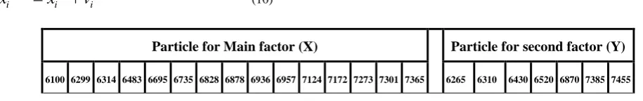
Later in second phase we used above obtained weights for forecasting formula and applied PSO on interval lengths to get optimized intervals and best forecast. For TAIFEX forecasting we obtained best particle shown below in Figure 2.
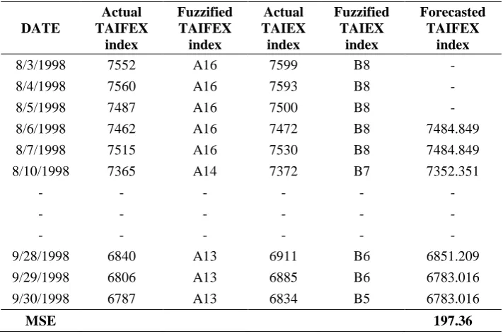
Forecasted Values for TAIFEX using proposed algorithm are shown below in Table 2. From Table 2 we can see that MSE of obtained forecast is 197.36.
We have compared our method with many previous methods, as shown in Table 3 below. From Table 3 we can see that proposed algorithm has less MSE, so better forecasting accuracy as compared to previous methods
7. Conclusion and Future Work
In this paper we have presented a two phase algorithm for fuzzy time series forecasting of TAIFEX index. Proposed algorithm uses GA and PSO in phase 1 and 2 respectively. In phase 1, we used genetic algorithm to adjust the weights for the fuzzy aggregation operation in (5). For adjusting the interval width, we have used PSO algorithm and simulated
Particle for Main factor (X) Particle for second factor (Y)
6100 6299 6314 6483 6695 6735 6828 6878 6936 6957 7124 7172 7273 7301 7365 6265 6310 6430 6520 6870 7385 7455
[image:5.595.57.515.638.710.2]Table 3: Comparison of MSE of different
methods with proposed method for TAIFEX
forecasting
.
Methods MSEQuantile based method (Jilani and Burney [29]) 3736.64 Lee, Wang and Chen [28] 249.61 Wang and Chen [30] 252.47
Proposed Method 197.36
the experiment with different values of the constants c1 and c2. The best partitioning is optimized where MSE is used as objective function. Using these techniques, we obtained MSE of Forecasting 197.36. A comparison of our proposed methods and other methods is given in Table 3.
In future work we aim to implement other nature inspired techniques for optimization in fuzzy time series forecasting algorithms so that we have better accuracy with low computational complexity.
8.
REFERENCES
[1] Q. Song, B. S. Chissom, Forecasting enrollments with fuzzy time series Part I, Fuzzy Sets and Systems, 54: 1-9.
[2] Q. Song, B. S. Chissom, Forecasting enrollments with fuzzy time series Part II, Fuzzy Sets and Systems, Vol. 62: pp. 1-8, 1994.
[3] Chen, S. M. 1996. Forecasting enrollments based on fuzzy time series, Fuzzy Sets and Systems, 81: 311-319.
[4] S. M. Chen, Forecasting enrollments based on high-order fuzzy time series, Cybernetics and Systems: An International Journal, Vol. 33: pp. 1-16, 2002.
[5] Chen, S. M. and Hsu, C.-C. 2004. A new method to forecasting enrollments using fuzzy time series, International
[6] K. Huarng, Heuristic models of fuzzy time series for forecasting, Fuzzy Sets and Systems, Vol. 123, pp. 369-386, 2002.
[7] K. Huarng, Effective lengths of intervals to improve forecasting in fuzzy time series, Fuzzy Sets and Systems, Vol. 12, pp. 387- 94, 2001.
[8] J. R. Hwang, S. M. Chen, C. H. Lee, Handling forecasting problems using fuzzy time series, Fuzzy Sets and Systems, Vol. 100, pp. 217-228, 1998.
[9] T. A. Jilani, S. M. A. Burney, C. Ardil, Fuzzy Metric Approach for Fuzzy Time Series Forecasting based on Frequency Density Based Partitioning, Proceedings of World Academy of Science, Engineering and Technology, Vol. 23, pp.333-338., 2007.
[10]S. Melike, K. Y. Degtiarev, Forecasting Enrollment Model Based on First-Order Fuzzy Time Series, Proceedings of World Academy of Science, Engineering and Technology, Vol. 1, pp. 1307-6884, 2005.
[image:6.595.120.476.128.364.2][11]S. Melike, Y. D. Konstsntin, Forecasting enrollment model based on first-order fuzzy time series, in proc. International Conference on Computational Intelligence, Istanbul, Turkey, 2004.
Table 2: Forecasted Values of TAIFEX
DATE
Actual TAIFEX
index
Fuzzified TAIFEX index
Actual TAIEX index
Fuzzified TAIEX
index
Forecasted TAIFEX
index
8/3/1998 7552 A16 7599 B8 - 8/4/1998 7560 A16 7593 B8 - 8/5/1998 7487 A16 7500 B8 - 8/6/1998 7462 A16 7472 B8 7484.849 8/7/1998 7515 A16 7530 B8 7484.849 8/10/1998 7365 A14 7372 B7 7352.351
- - - - - - - - - - - - 9/28/1998 6840 A13 6911 B6 6851.209 9/29/1998 6806 A13 6885 B6 6783.016 9/30/1998 6787 A13 6834 B5 6783.016
[12]S. M. Chen, J. R. Hwang, Temperature prediction using fuzzy time series, IEEE Transactions on Systems, Man, and Cybernetics-Part B: Cybernetics, Vol. 30, pp.263-275, 2000.
[13]L. W. Lee, L. W. Wang, S. M. Chen, Handling forecasting problems based on two-factors high-order time series, IEEE Transactions on Fuzzy Systems, Vol. 14, No. 3, pp.468-477, 2006.
[14]T. A. Jilani, S. M. A. Burney, M-factor high order fuzzy time series forecasting for road accident data, In IEEE-IFSA 2007, World Congress, Cancun, Mexico, June 18-21, Forthcoming in Book series Advances in Soft Computing, Springer-Verlag, 2007.
[15]T. A. Jilani, S. M. A. Burney, C. Ardil, Multivariate high order fuzzy time series forecasting for car road accidents, International Journal of Computational Intelligence, Vol. 4, No. 1, pp.15-20., 2007.
[16]T.A. Jilani, S.M.A. Burney, A refined fuzzy time series model for stock market forecasting, Physica-A 387 (2008c) 2857-2862.
[17]I-H. Kuo, S.-J. Horng, T.-W. Kao, T.-L. Lin, C.-L. Lee, Y. Pan, An improved method for forecasting enrollments based on fuzzy time series and particle swarm optimization, Expert Systems with Applications 36(3), (2009) 6108–6117
[18]Y.-L. Huang, S.-J. Horng, M. He, P. Fan, T.-W. Kao, M. K. Khan, J.-L. Lai, I-H. Kuo, A hybrid forecasting model for enrollments based on aggregated fuzzy time series and particle swarm optimization, Expert Systems with Applications 38(7), (2011) 8014–8023
[19]J.-I. Park, D.-J. Lee, C.-K. Song, M.-G. Chun, TAIFEX and KOSPI 200 forecasting based on two-factors high-order fuzzy time series and particle swarm optimization, Expert Systems with Applications 37(2), (2010) 959–967
[20]T.A. Jilani, S.M.A. Burney, U. Amjad and T. A. Siddiqui., A Particle Swarm Intelligence based Fuzzy Time Series Forecasting Model. International Journal of Computer Applications 38(10), (2012) 47-52
[21]Jilani T. A., Nikol Mastorakis, Usman Amjad (2012), “ A Hybrid Genetic Algorithm and Particle Swarm Optimization Based Fuzzy Time Series Model TAIFEX and KSE-100 Forecasting”, NAUN-First International Confernce on Biological Inspired Computation, University of Algaro, Portugal, 22-24, May-2012.
[22]Jilani T. A., J. Jaffar, Usman Amjad, H. Saima (2012), “An Improved Heuristic-Based Fuzzy Time Series Forecasting Model Using Genetic Algorithm”, ICCIS-2012, Petronas, Malaysia.
[23]L. A. Zadeh, "Fuzzy sets,” Information and Control, vol. 8, 1996, pp. 338-353.
[24]Q. Song, B. S. Chissom, Fuzzy time series and its models, Fuzzy Sets and Systems, Vol. 54, pp. 269-277, 1993.
[25]Goldberg D.E., 1989. Genetic algorithm in search, optimization, and machine learning, Addison-Wesley, Massachusetts.
[26]Goldberg D.E., Korb B., Deb K., 1989. Messy genetic algorithms: motivation, analysis, and first results, Complex Systems 3 (5), pp.493–530.
[27]J. Kennedy and R. Eberhart. Swarm Intelligence. Morgan Kaufmann Publishers, Inc., San Francisco, CA, 2001.
[28]Lee L.-W., Wang L.-H., Chen S.-M., 2007. Temperature prediction and TAIFEX forecasting based on fuzzy logical relationships and genetic algorithms, Expert Systems with Applications 33, 2007, pp. 539- 550.
[29]T.A. Jilani, S.M.A. Burney, C. Ardil, A New Quantile Based Fuzzy Time Series Forecasting Model, International Journal of Intelligent Systems and Technologies 3 (4), (2008d), pp. 201-207.
![Table -5, the forecasted value is calculated using (Jilani, Burney [14]):](https://thumb-us.123doks.com/thumbv2/123dok_us/8101504.788017/3.595.60.274.548.730/table-forecasted-value-calculated-using-jilani-burney.webp)