Munich Personal RePEc Archive
Valuing Access to U.S. Public Lands: A
Unique Pricing Experiment
Aadland, David and Anatchkova, Bistra and Grandjean,
Burke and Shogren, Jason and Simon, Benjamin and Taylor,
Patricia
University of Wyoming
1 April 2008
VALUING ACCESS TO U.S. PUBLIC LANDS: A UNIQUE PRICING EXPERIMENT
April 22, 2008
1. Introduction
This paper reports the findings of a unique nation-wide experiment to price access to U.S.
federal lands. The Federal Lands Recreation Enhancement Act of 2004 mandated a new
recreation pass (hereafter, the NRP) to replace the Golden Eagle Passport (GEP) and the
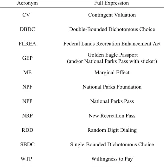
National Parks Pass. (For a list of acronyms used in this paper, see Table 1.) The NRP, similar
to the GEP, covers all federal lands that charge an entrance or access fee for recreational use.
This includes units administered by the National Park Service, many sites administered by the
U.S. Forest Service, and some locations administered by other federal agencies.
Our economic and survey research team undertook an economic analysis of the new pass
program and submitted a price recommendation to federal land management agencies in the fall
of 2006. The project was completed under the constraint that the NRP should “provide
convenient access, at a fair price, to federal recreation sites that charge fees….and should at least
allow the government to break even in the sense that, on average, the sale of the [NRP] does not
result in a revenue loss relative to the revenue that would be received absent the ability to
purchase an annual pass.”1 After receiving our analysis and price recommendation, the U.S.
Departments of Agriculture and the Interior announced that the price for the annual NRP would
be set at $80; the new pass went on sale in January 2007.
Here we describe the methodological and economic issues associated with assisting federal
land management agencies to determine an appropriate price for the new pass. We used
contingent valuation (CV) methods to help determine an appropriate price for the NRP. CV and
1
This should be recognized as a political constraint on the price-setting exercise; as stipulated by the sponsoring agencies, “revenue neutrality” was defined in relation to revenues absent any pass, not in relation to revenues from existing passes. There are other possible policy issues associated with pass pricing (e.g., public education,
other stated preference valuation methods have made significant in-roads into public
decision-making over the past two decades. Federal policymakers use the value estimates to help guide
their decisions for a range of topics like water quality protection, air quality improvements,
watershed and ecosystem protection, and reduced human health risk (see for example Brown,
Champ, and Boyle, 2004).
In the present application, an innovative experimental design allows us to contrast the
hypothetical purchasing decisions of survey respondents with the actual purchasing decisions of
households. As a result, we are less open to a major criticism of contingent valuation analysis—
hypothetical bias. Hypothetical bias exists when people misstate their actual willingness to pay
(WTP) in a survey. In our analysis, we account for hypothetical decision-making because we
are able to calibrate our new price estimates to the actual purchasing decisions of households.2
Unlike most other non-market valuation exercises, we have a real benchmark – the GEP.
The GEP entitled households to basically identical access to public lands as the NRP and had
been offered at $65 since 2000. Using past GEP sales figures and the reported purchasing
decisions of households within our sample, we are able to estimate three distinct components of
hypothetical bias. The total degree of hypothetical bias in our sampling of the U.S. general
population (a Random Digit Dialing sample) implies that NRP revenues estimated directly from
the uncalibrated household survey responses would be higher than actual revenues by a factor of
16. The total bias using our sampling of recent pass purchasers (a sample obtained from the
2
The topic of hypothetical bias has triggered a large literature in non-market valuation research (see Murphy et al., 2005). Research can be grouped into two broad categories: ex ante or ex post. Ex ante methods frame the valuation question so as to make it more “real” to the person asked the valuation question, or they provide additional
National Parks Foundation) is much lower and even slightly negative. This finding supports
previous research in the area of non-market valuation3, which shows that market experience is an
important indicator of people’s ability to accurately identify and state their true valuation for
public and environmental goods (e.g., List and Shogren, 1998; List and Gallet, 2001; Cherry et
al., 2003; Murphy et al., 2005; and Cherry and Shogren, 2007).
2. Background
The Federal Lands Recreation Enhancement Act (Public Law 108-447, the FLREA), which
was signed into law on December 8, 2004, established a new recreation pass to replace the
existing GEP and National Parks Pass (NPP). The FLREA called for a pass to provide
convenient and fairly priced access to federal recreation sites that charge fees; to provide
opportunities for education on federal lands; to provide support for public lands; and to develop
partnerships with organizations that support recreation and stewardship on public lands.
This new pass (the NRP) covers the entrance fees for units administered by the National Park
Service and the U.S. Fish and Wildlife Service, as well as standard amenity fees for developed
areas administered by the U.S. Forest Service, the Bureau of Land Management, and the Bureau
of Reclamation. Fee areas generally include visitor centers or other developments with certain
basic facilities (e.g., designated parking, restrooms, etc.). Like the passes it replaces, the new
pass does not cover any expanded amenity fees for such things as reservation services or
developed campgrounds and boat launches. When appropriate, pass holders will also continue to
3
pay special recreation permit fees such as those for motorized recreational vehicle use,
recreational events, and group activities.
The NRP is similar to the earlier GEP. The GEP was introduced in 1965, at a price of $7 per
year. By 1997 its price had risen to $50; by 2000 the price was $65. Like the NRP, the GEP
provides entrance for the passholder (and other occupants of a private vehicle) to virtually all
federal lands that charge a fee.4 The year 2000 saw the introduction of the NPP, sold for $50 and
providing entrance only to those federal lands administered by the National Park Service. For an
additional $15, a sticker could be purchased and affixed to the NPP to make it equivalent in all
respects to the GEP (and therefore, essentially equivalent to the NRP). Throughout this paper,
“GEP” refers to either the Golden Eagle Passport or the National Parks Pass with sticker, while
“NPP” refers to the National Parks Pass without the sticker. Sales of the GEP and the NPP were
discontinued in January of 2007 when the NRP was introduced.
3. Economic Analysis
Our economic analysis begins with the assumption that by stating their WTP for the NRP,
households are revealing their optimal choice for expected number of visits to federal recreation
sites. This assumption provides a convenient method for calculating expected pass and gate
revenues. All households with a maximum WTP above the price of the NRP will purchase the
pass and contribute exclusively to pass revenues; all households with a maximum WTP that is
below the price of the NRP will instead pay at the gate and contribute exclusively to gate
4
revenues. We can then evaluate how various NRP prices will impact total pass and gate revenues,
and whether the prices satisfy the “revenue neutrality” constraint mentioned in Section 1.
The value of the NRP is derived from both use and non-use sources. The NRP provides
access to recreation at federal sites, without paying daily entrance or usage fees. We refer to this
as use value, which can in turn be separated into convenience and economic value. Convenience
refers to the reduced transaction costs associated with using the NRP rather than having to make
separate payments for each entrance fee.5 Economic value is derived from the expected cost in
entrance fees, given the number of planned visits to recreation sites and the current entrance fee
structure.6 The NRP may also provide households with a sense of satisfaction in helping to fund
the creation and maintenance of federal recreation sites that may be used by others. We refer to
this non-use value as stewardship value.
In deciding whether to purchase the NRP, households weigh all the benefits and costs. The
benefits include convenience, economic value, and possible stewardship motives. The relevant
cost is the price of the pass. The household’s decision is straightforward – if the total benefits
outweigh the private costs, purchase the pass; otherwise, pay the gate fees. To better understand
this decision, we undertook a CV experiment designed to simulate the actual market environment
and NRP purchasing decisions.
5
We note that some may find an offsetting inconvenience in having to remember to bring the pass for each visit. In concept, some of the values associated with “convenience” also accrue to the federal government if having a pass reduces wait times at entrance stations, allowing fee collectors to work more efficiently.
6
3.1 Hypothetical Bias
A fundamental concern of any CV study is hypothetical bias. Respondents have a
well-established tendency to state willingness to pay values that are significantly greater than those
revealed in real-market interactions (e.g., Diamond and Hausman, 1994; Harrison and Rutström,
2006). While different methods have been proposed to obtain more accurate WTP values from
non-market valuation surveys (Boyle, 2003), our study has a built-in mechanism to calibrate
hypothetical WTP values with real choices. We take advantage of the fact that the NRP is nearly
identical to the existing GEP, which was previously sold in the marketplace. Our survey design
(described in more detail below) uses revealed-preference data from the GEP market to generate
calibration factors for three components of hypothetical bias within our survey sample. We use
these estimated calibration factors to adjust WTP values from the survey so they are consistent
with the actual purchasing decisions of households. The details of this calibration exercise are
described in Sections 5.2 through 6.1.
3.2 Calculating NRP and Gate Revenues
Initially, we assume households are motivated to purchase the NRP based solely on its
economic value. That is, people purchase the pass if it reduces the total planned entrance
expenses for visitation to federal recreation sites and do not place any value on convenience or
stewardship. With this assumption (which we relax later), it is straightforward to use our
estimated WTP values to project the NRP revenue and gate revenue associated with various NRP
fee levels. NRP revenue is defined as the revenue generated directly from sales of the NRP.
Gate revenue is the revenue generated from on-site entrance fees at federal recreation sites.
To further clarify, consider the case in which a household’s maximum WTP for the NRP is
nothing to gate revenues.7 Conversely, if the household’s maximum WTP is less than the cost of
the NRP, the household will not purchase the pass and instead pay at the gate. If the household’s
WTP for the NRP is driven by economics, the most they would be willing to pay for the pass
would be the exact amount they expect to spend at the gate. This produces a straightforward
method for calculating NRP and gate revenues:
NRP Revenue =
∑
≥NRPPrice WTP
ice Pr
NRP (1.1)
Gate Revenues =
∑
<NRPPrice WTP
WTP (1.2)
Total NRP revenues are calculated by multiplying NRP price by the total number of
households with a maximum WTP greater than the price (i.e., all households that would purchase
the pass). Total gate revenues are calculated by summing up maximum WTP for all households
with WTP less than the NRP price (i.e., all households that would not purchase the pass and
instead pay at the gate). This method for estimating total gate revenues assumes that (i)
households do not systematically over- (or under-) estimate the number of trips to federal
recreation sites, and (ii) they do not purchase the pass for convenience or stewardship purposes.
The effect of relaxing these assumptions is considered at the end of Section 6.2.3.
4. Survey Design
Our goal with the survey was to link the NRP valuation exercise to real choices and real
outside options; respondents answered the new valuation question after thinking about the status
7
quo and their familiarity with the NPP and GEP. Our intent was to keep the survey realistic,
simple, and quick while still generating reasonable value estimates. Given time constraints and
the scale of the project a face-to-face survey was infeasible. Instead, we conducted a nationwide
telephone survey between February and April of 2006.
The survey sample consisted of two independent strata. The first stratum was sampled using
a national Random Digit Dialing (RDD) draw of households with landline telephones. To
enhance the precision of estimates from this part of the sample, it was pre-stratified by the 9
major geographic divisions defined by the U.S. Bureau of the Census, and post-stratified to
reflect Census Bureau distributions by geographic division, household income, Hispanic origin,
and racial identification. By design, this sample of 1,799 responding RDD households represents
the roughly 110 million households in the U.S. with landline phones, except for about 30,000
that fall into the second stratum. The second stratum was randomly sampled from a population
list of telephone numbers for households known to the National Parks Foundation (NPF) to have
purchased a National Parks Pass (with or without a sticker) between April 2004 and March 2005
(i.e., from one to two years prior to the survey). This sample was also pre-stratified by
geographic division, and the 1,974 responding NPF households were weighted to match the
geographic distribution of the NPF population list.
The total sample size across both strata was 3,773 households. Within-household sampling
was not undertaken, because the relevant unit of analysis is the household. The NRP (like the
GEP and NPP) is not an individual pass; rather, it entitles the members of a household traveling
together to access federal lands for recreation. Therefore, any willing adult respondent in each
With total sales of approximately half a million passes per year, the NPF population list of
only 30,629 households covers just a small subset of NPP and GEP purchasers one to two years
earlier; obviously, it covers an even smaller fraction of all U.S. households. The NPF sampling
frame mainly represents households that purchased the pass on-line. It omits most of the roughly
50,000 annual purchasers of the GEP, except to the (unknown) extent that those on the NPF list
may have purchased the $15 sticker that upgrades the NPP to the GEP. Fortunately, our interest
in the NPF sample is not predicated on claiming it represents all pass purchasers. Rather, the
NPF sample reflects a small but noteworthy group of supporters of the national parks (who tend
to be familiar with the passes), while the RDD sample is designed to represent the full spectrum
of the population of U.S. households (the majority of whom are unfamiliar with the passes).
Both samples were screened, through questions asked early in the survey, to eliminate from
our analysis those households in which anyone qualified for a Golden Age or Golden Access
Passport. These lifetime passes, available only to senior citizens and the disabled, effectively
remove a household from the market for an annual GEP, NPP, or NRP. As stipulated by the
sponsoring agencies, households that had not visited any federal recreation lands in the past two
years were also screened out of the analysis, on the assumption they would not be part of the
relevant market either. Protest households (those that said they would not accept the NRP for
free) were excluded as well, for the same reason. After all screening, the RDD sample provided
462 cases for analysis and the NPF sample provided 1,461 cases.8
8
The survey questionnaire began with an introduction, screening questions, and a short series
of items about the household’s recent recreational experiences on federal lands. (The complete
questionnaire is available from the authors on request [and is provided as an attachment here for
use by the reviewers].) The interviewer then asked whether the respondent was aware of the NPP
or GEP. If the answer was “YES”, the respondent was asked whether the household had
purchased the NPP or GEP in the past 12 months.
The next section of the questionnaire provided a short description of the NRP followed by
the valuation question, which asked whether the household would be willing to buy the NRP at a
randomly selected bid value. For some respondents, the random bid value was the current GEP
price, which allows us to compare hypothetical purchasing decisions to real purchasing
decisions. To more precisely pinpoint the valuation distribution, the interviewer then asked a
follow-up question. If the respondent was willing to purchase the NRP at the first bid price, we
increased the price by a randomly set amount and asked again; if not, we lowered the price and
asked again.
The final section of the questionnaire asked a series of socio-demographic questions
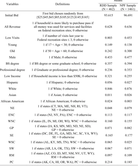
including age, education, race, and household income. Table 2 presents the full set of variables
used here, with definitions and descriptive statistics.9 We turn now to the econometric analysis
of the survey data.
by Dorofeev and Grant, 2007, p. 105). Further details regarding survey design, sampling, and weighting can be found in (reference deleted for anonymity in the review process).
9 Although not explicitly modeled here, a potential source of explanatory power is the distance to nearby federal
5. Econometric Analysis
We break the econometric analysis into three sections. In Section 5.1, we present the model
to estimate overall WTP for the NRP. Section 5.2 defines the model used to estimate the degree
of hypothetical bias in terms of increased probability that a stated-preference household will
purchase the pass at $65. Finally, in Section 5.3, we describe how to use the two models to
translate the probability measure into a dollar-denominated measure of hypothetical bias. This
scaling factor, which we term “internal” hypothetical bias, is one of three components that we
use to calibrate the WTP estimates to the actual purchasing decisions of households. The other
two (“awareness” bias and “external” hypothetical bias)10 are examined in Section 6.
5.1 Overall WTP Model
Our first econometric model estimates WTP for the NRP, which in turn can be used to
forecast pass and gate revenue at various NRP prices. We use an interval regression model that
follows directly from the double-bounded dichotomous-choice (DBDC) survey design described
above (Hanemann et al., 1991). An interval regression is an ordered probit model with variable
and known cut points (Woolridge, 2002).
We start by writing the empirical model in terms of a household’s maximum WTP for the
NRP, which is indirectly derived from the utility of visiting federal recreation sites:
) X
exp(
WTPi = ′iβ+εi , (3)
10
Awareness bias refers to the fact that all survey respondents were made aware of the NRP and its features before being asked about their willingness to purchase it, whereas a substantial fraction of households in the general population would likely remain unaware of the NRP’s existence (as is true of the GEP and NPP, according to our survey) and therefore would not have the opportunity to purchase it. External hypothetical bias refers to the
where WTPi is the latent willingness to pay for the NRP; Xi is a vector of explanatory variables; β
is a vector of coefficients; εi is a mean-zero Gaussian error term with variance σ2; and i = 1,..,N
indexes households in a sample of size N. The exponential functional form guarantees the
predicted WTP will be non-negative. Given expression (3), the probability of purchasing the
pass is represented as
))) b ln( X ( 1 ( ) b WTP Pr( ) 1 y Pr(
Pi i i i ′iβ− i
σ Φ = ≥ =
=
= , (4)
where Φ is the standard normal cumulative density function, yi= 1 if the household purchased
the pass, yi = 0 if the household did not purchase the pass, and bi is the proposed price of the
NRP. The initial bids are chosen at random from the following bid vector (which we developed
using focus groups):
b= ($25, 45, 65, 85, 105, 125, 145, 165). (5)
Table 3 shows the percent of the RDD and NPF samples that respond “YES” to the initial
bids. As expected, the percent responding “YES” generally declines as the bids increase in
value, and the NPF respondents are more likely to say “YES” at every bid price. As described in
Section 4, we follow the initial bid with a second one, randomly selected from either
bH = (b+$20, 2b-$5) if the respondent accepts the first bid or bL = (b-$20, 0.5(b+$5)) if the
respondent declines.11 If a respondent answers “NO” to both bids, we ask another follow-up
11
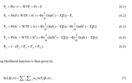
question with a bid equal to zero, in order to identify protest bidders. Given (3), the probabilities
of purchasing a pass within each possible range of prices are
0 ) 0 WTP Pr(
Pi1= −∞< i < = (6.1)
i 1 i L i L i i 2
i (ln(b ) X )) P
1 ( ) b WTP 0 Pr(
P − ′β −
σ Φ = ≤ ≤
= (6.2)
)) X ) b (ln( 1 ( )) X ) b (ln( 1 ( ) b WTP b Pr(
Pi3 iL i i i i iL − ′iβ
σ Φ − β ′ − σ Φ = ≤ <
= (6.3)
)) X ) b (ln( 1 ( )) X ) b (ln( 1 ( ) b WTP b Pr(
Pi4 i i Hi Hi i i − ′iβ
σ Φ − β ′ − σ Φ = ≤ <
= (6.4)
) P P P P ( 1
Pi5 = − i1 + i2 + i3+ i4 . (6.5)
The log likelihood function is then given by
∑ ∑
= = ω β σ= σ β N 1 i 5 1
j ijlnPij( , )
) , ( L
ln , (7)
where ωij is a binary variable equal to one if household i chooses category j. We choose β and σ
to maximize the likelihood function. With estimates of β and σ in hand, we form WTP estimates
[image:15.612.97.561.140.432.2]for every household in the sample, and in turn the NRP and gate revenue functions.
Table 4 presents the results from the DBDC model. We analyze the RDD and NPF samples
separately throughout, because the two populations are substantially different in their
demographic characteristics (e.g., NPF respondents tend to be older, with more education and
higher income), in their visitation to federal recreation sites, and of course, in their recent
purchases of federal recreation passes. Protest households (i.e., those who refuse the pass for
free) are excluded from all analyses, based on the original screening decision to exclude
households that are unlikely to participate in the market for the NRP. As compared to the rest of
the sample, protest households (N=67 for RDD; N=30 for NPF) tend to be older, less educated,
lower income, less likely to be white, and more likely to reside in states in the northeast (NJ, NY
and PA) or great plains (IA, KS, MN, MO, ND, NE and SD).
We incorporate heteroscedasticity into the econometric model because the WTP bid intervals
vary across households. Recall that half of our follow-up bids are either half or twice the initial
bid, so higher initial bids tend to be associated with larger WTP intervals. We use the initial bid
to proxy for interval width and model the heteroscedasticity as
) b
exp( 0 1 i
2
i = α +α
σ . (8)
As shown in Table 4, the test statistic for heteroscedasticity is large in the NPF sample, leading
us to reject the null of homoscedastic errors there, but not in the RDD sample.
Mean and median WTP figures are presented at the bottom of Table 4. The mean and
median WTP values for the RDD sample are approximately $42 and $35, indicating a WTP
distribution that is slightly skewed toward higher WTP values. The mean and median WTP
values for the NPF sample are both approximately $95, an average substantially higher than in
the RDD sample, which is expected given that the NPF sample is comprised of recent pass
purchasers.12 Next, we consider hypothetical bias.
12
5.2 Modeling Internal Hypothetical Bias13
We now describe the econometric procedure to calibrate estimated WTP to be consistent
with stated rates of GEP purchases from within our two survey samples. We designed our
valuation experiment to account for hypothetical bias by comparing hypothetical decisions to
buy the NRP (at a bid equal to $65) with actual decisions to purchase the existing GEP, which
has been sold for $65 in the marketplace since 2000. Assuming households are accurately
stating whether or not they purchased the GEP within the immediately preceding 12 months, this
internal calibration should result in WTP and revenue estimates that more nearly reflect the
actual purchasing decisions of households in the general U.S. population.
To estimate the degree of internal hypothetical bias in the survey data, we specify a probit
model with a dummy variable to capture the difference between hypothetical and actual
purchasing decisions. Within the RDD and NPF samples taken separately, we pool data from
two distinct subsamples—the stated preference and the revealed preference subsamples. The
revealed preference subsample includes every household who knew of the $65 GEP, whether or
not they had purchased one. The stated preference subsample includes every household that was
unaware of the GEP and received an initial bid of $65 for the NRP, whether or not they said
“YES” to that bid. Protest households (who refused the pass for free) are excluded from the
analysis.14
The underlying economic model is similar to (3) but modified to incorporate hypothetical
bias
13
The estimation of what we call “internal” hypothetical bias in this section follows Aadland and Caplan (2003). Because our estimation of internal hypothetical bias captures any difference between stated and revealed
preferences, it will include other differences such as strategic bias. Strategic bias occurs when households intentionally say ‘NO’ to an acceptable bid in order to encourage policymakers to set a lower price.
14
) X exp( ) SP exp( ) SP X exp(
WTPi = ′iβ+δ⋅ i +εi = δ⋅ i ′iβ+εi , (9)
where WTPi is unobserved willingness to pay for either the GEP or the NRP, SPi is a dummy
variable equal to one for the stated-preference subsample and zero for the revealed-preference
subsample, and δ is the hypothetical bias coefficient. Analyzing the RDD and NPF samples
separately, we form the probability (Pi) that the ith household purchases the pass at a price of $65:
))) 65 ln($ SP X ( 1 ( ) 65 $ WTP Pr(
Pi i ′iβ+δ⋅ i−
σ Φ = ≥
= . (10)
Let yi= 1 indicate the household purchased the pass (either hypothetical or real), and let yi = 0
indicate they did not purchase the pass. This is a probit model with (log) likelihood function
[
]
∑
= + − − = δ β N 1i yiln(Pi) (1 yi)ln(1 Pi)
) X , y | , ( L
ln . (11)
The coefficients β and δ are only identifiable up to the scale factor (1/ ). Because β and δ
only show up in the likelihood function as a ratio with (i.e., (β/ ) and (δ/ )) and the price is
fixed at $65, it is impossible to disentangle the ratios and obtain individual estimates of β, δ and
. However, the marginal effects, which measure the change in probability for a one unit change
in the explanatory variables (X or SP), only depend on the identifiable ratios. For the average
(
X( / ) ( / )) (
X( / ))
) 0 SP , X | 1 y Pr( ) 1 SP , X | 1 y Pr( σ β ′ Φ − σ δ + σ β ′ Φ = = = − = = = Δ (12)where a bar over the variable represents its average value. This coefficient is defined in terms of
increased (or decreased) probability of pass purchase. In the next section, we describe how to
translate Δ into a WTP scale factor using the baseline DBDC model.
5.3 Translating Internal Hypothetical Bias from a Probability into Dollars
The coefficient of hypothetical bias Δ in expression (12) is measured in terms of probability
the pass is purchased. Although this provides evidence of hypothetical bias, it does not allow
household WTP and welfare measures to be directly adjusted to reflect revealed preferences.
Furthermore, the probit model shown in expression (10) does not identify a dollar amount of
hypothetical bias because the bids are not varied (i.e., the bid is fixed at $65). Fortunately, the
DBDC model described in Section 5.1 uses the entire bid vector and allows us to identify
household WTP.
We use the normal distribution along with estimates of β and $65 to
back out the WTP hypothetical bias scale factor consistent with Δ for the average household.15
This is accomplished by solving for δ (given estimates of β, , and Δ) from the following
equation:
15
))), 65 ln($ X ( ˆ 1 ( ))) 65 ln($ X ( ˆ 1 ( ) 65 $ WTP Pr( ) 65 $ WTP
Pr( SP RP
− β ′ σ Φ − − δ + β ′ σ Φ = > − > = Δ (13)
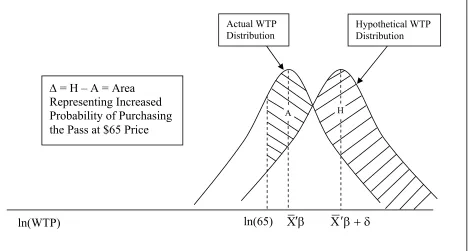
Figure 1a illustrates the procedure for identifying exp(δ), the WTP scale factor for hypothetical
bias for the RDD sample, while Figure 1b illustrates the procedure using the NPF sample. The
procedure is the same for each sample, but the figures are drawn separately to reflect the position
and shape of the empirical WTP distributions for each sample.
We start with our estimate of hypothetical bias, Δ, which is measured in terms of the
increased probability the NRP is purchased. This value is estimated using the method outlined in
Section 5.2 and is represented by the etched area in Figure 1a. (In Figure 1b it is the difference
between areas H and A.) The area under the hypothetical WTP distribution to the right of
ln($65) is the probability that a household will hypothetically accept a $65 bid for the NRP; the
area under the actual WTP distribution to the right of ln($65) is the probability that a household
will actually purchase the NRP at a $65 price. The difference between the two probabilities is Δ.
Assuming a normal distribution, we then back out the unique value of δ that positions the
hypothetical WTP distribution to be consistent with Δ and the standard deviation . Finally, we
use the corresponding WTP scale factor, exp(δ), to form the internally calibrated WTP estimates
[WTPi / exp(δ)] that more accurately reflect actual purchasing decisions of households.
We now turn our attention to the results from the hypothetical bias model outlined above,
estimated separately for the RDD and NPF samples. The first row of Table 5 presents the
coefficient and marginal effect (ME) estimates for hypothetical bias. In both samples, the
hypothetical bias coefficients are positive and statistically significant. The ME estimates
12.6 percentage points more likely to purchase a hypothetical $65 NRP than similar
revealed-preference households are to have purchased the actual $65 GEP. The control variables include
demographics such as age, gender, education, race and region.
As discussed above, the estimates of Δ need to be translated from a probability into a WTP
scale factor (i.e., we need to map our estimates of Δ into estimates of exp(δ) for the purpose of
calibrating the WTP estimates for hypothetical bias). To accomplish this, we use the baseline
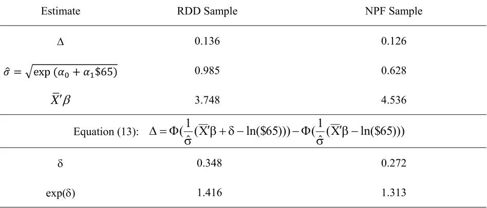
DBDC estimates reported in Table 4. The estimated value for the hypothetical bias calibration
factor, exp(δ), is approximately 1.4 and 1.3 for the RDD and NPF samples. Table 6 reports the
details for this calculation. Put differently, the dollar values for WTP in the RDD and NPF
samples need to be reduced by 40% and 30% to be consistent with the observation that
stated-preference households are 13.6 and 12.6 percentage points more likely than revealed-stated-preference
households to purchase a pass at $65. The revenue functions reported below are therefore scaled
by exp(δ) to more accurately reflect actual purchasing decisions.
However, these estimates of hypothetical bias are likely to be lower bounds on the true total
bias in the population. To estimate internal hypothetical bias, the sample was partitioned
according to whether respondents were aware of the GEP (revealed-preference households) or
not aware of the GEP (stated-preference households, if they received a $65 bid for the NRP). If
lack of awareness of the GEP is associated with a lower propensity to visit federal recreation
sites (and therefore a lower WTP for the NRP), then our stated-preference households are, all
else equal, less likely to hypothetically purchase a pass at any given price. This will lead to an
underestimate of internal hypothetical bias by the method just described. Accordingly, we next
augment our calibration to include an explicit adjustment for awareness bias and a final
6. Estimated Revenue Functions
In this section, we describe the calibration process and present the resulting NRP and gate
revenue functions. We calculate both parametric and non-parametric estimates of the revenue
functions. The parametric estimates of the revenue functions are based on the DBDC model and
methods outlined in Section 5.1. The non-parametric estimates of the revenue functions are a
direct reflection of households’ “YES” or “NO” responses to the various bids presented in the
CV analysis. For simplicity, we focus on the non-parametric estimates and make the parametric
estimates available upon request.16
6.1Calibration for Awareness, Internal, and External Hypothetical Bias
All the revenue functions are first calibrated for awareness bias. Approximately 50% of the
RDD sample and 4% of the NPF sample were unaware of both the NPP and GEP.17 Assuming
the NRP is marketed in a similar manner, we expect similar fractions of the respective
populations would not purchase the NRP at any price, simply because they would not learn of its
existence. To account for this in our population revenue projections, we calculate NRP revenues
in the sample by summing NRP revenues only for those who were aware of either the NPP or the
GEP and have a maximum WTP that is higher than the proposed NRP price. We then scale that
amount up to the appropriate population size. Estimated gate revenues do include households
16
The primary difference between the estimates is that the non-parametric model has more success predicting the small number of households that place themselves at the tails of the WTP distributions (see Greene (2003), page 685). Although the revenue functions tend to have a similar shape, the peak revenue occurs at a substantially lower price for the parametric estimates.
17
who were unaware of both the NPP and the GEP, under the assumption such households would
continue to visit federal recreation sites and pay gate fees.
After adjusting for awareness bias, we calibrate sequentially for what we term internal and
external hypothetical bias. The internal calibration procedure uses the sample RDD and NPF
survey data and is outlined in Sections 5.2 and 5.3. Unlike other valuation studies, however, our
research design permits a further important adjustment: using external information to calibrate
our WTP estimates against actual purchasing decisions in the aggregate. Our external calibration
uses outside information on recent pass revenues to project future pass revenues and then
matches them to projected NRP revenues. As a consequence, the external calibration adjusts for
any remaining hypothetical bias not addressed by the awareness or internal hypothetical bias
adjustments.
Based on recent pass sales, we project that at a price of $65, NRP revenues should be
approximately $30 million and $1 million for the RDD and NPF populations.18 After
adjustments to WTP for awareness bias and internal hypothetical bias, we then scale the
corresponding NRP revenues to match these figures. Because gate revenues are calculated from
NRP revenues, they are automatically calibrated in a similar fashion.
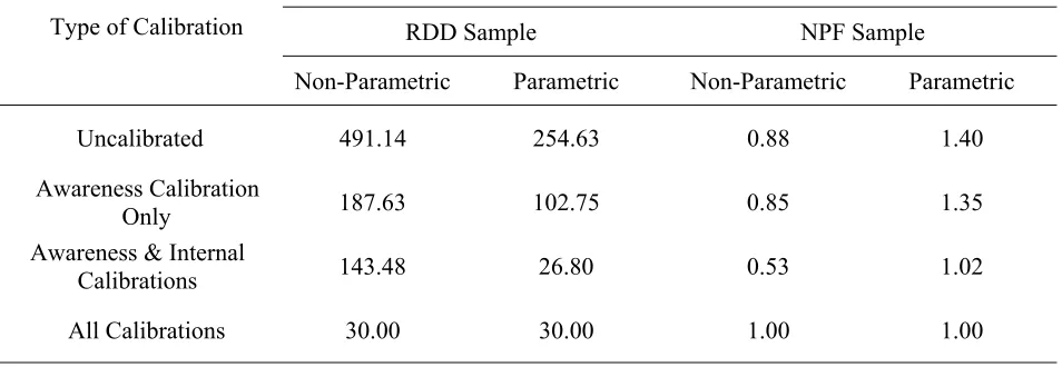
Table 7 presents the magnitudes of all three types of calibration factors. Panel A shows the
projected NRP revenues based on various assumptions about awareness and hypothetical bias in
the relevant populations. Panel B presents total scaling factors and their decomposition into
18
awareness bias, internal hypothetical bias and external hypothetical bias. In calculating the total
bias, the decomposed terms are multiplied together, rather than added, to be consistent with the
multiplicative hypothetical bias term in equation (9). By decomposing the total bias in a
multiplicative fashion, each individual bias term retains the interpretation of a ‘scaling factor’.
The scaling factors in Panel B are calculated using the revenue projections in Panel A. First,
the scaling factors for awareness bias are calculated by taking the ratio of predicted NRP
revenues at $65 (assuming all households in the population will be made aware of the NRP) to
the predicted NRP revenues at $65 (assuming that households in the population will be aware of
the NRP at the same rate as our sample was aware of the GEP or NPP). Second, maintaining the
correction for awareness bias, the internal hypothetical bias scaling factor is calculated by taking
the ratio of predicted NRP revenues at $65 (without a correction for internal hypothetical bias) to
predicted NRP revenues at $65 (after scaling WTP by exp(δ)). Finally, the external bias factor is
calculated by taking the ratio of projected revenues at $65 (with adjustments for awareness and
internal hypothetical bias) to the benchmark revenues mentioned above ($30 million and $1
million for the RDD and NPF populations).
Panel B of Table 7 shows the total degree of awareness and hypothetical bias. Using the
RDD sample and the non-parametric forecasts, the uncalibrated NRP revenues are approximately
16 times higher than the calibrated data would suggest. Using the parametric forecasts, the bias
in the uncalibrated RDD results is only half as large, and it is completely eliminated by just the
awareness and internal calibrations.
The total bias using the NPF sample is much lower (perhaps negligible for some purposes),
and even slightly negative in the non-parametric case. This suggests the overall hypothetical
NPF sample. The result also confirms previous empirical and meta-analysis research that market
experience helps mitigate valuation biases (e.g., List and Shogren, 1998; List and Gallet, 2001;
Cherry et al., 2003; Murphy et al., 2005; Cherry and Shogren, 2007).
6.2 Projected Revenue Functions
Next we present non-parametric, calibrated estimates for NRP and gate revenues.19
6.2.1 NRP Revenue
As shown in Table 8,the NRP revenue functions reach maximums at approximately $25 and
$45 for the RDD and NPF samples. For the RDD sample, NRP revenues drop sharply at $45 and
then level off up to $105, after which pass revenues again begin to fall more rapidly. In the NPF
sample, the decline in pass revenues after the peak is steady out to $265. The degree of
sensitivity of NRP revenues to price reflects the elasticity of the underlying demand curve for the
NRP. Recall, all these revenue functions are calibrated for awareness, hypothetical and external
bias as described in Section 6.1.
6.2.2 Gate Revenue
Table 8 also shows gate revenues. We project the level of gate revenues based on
households’ maximum WTP for the NRP (i.e., the most households should be willing to pay for
the NRP is the amount they expect to spend at the gate). At low NRP prices, gate revenues are
19 We calculate the non-parametric revenue functions by assuming the household’s true WTP is at the midpoint of
relatively low and consist primarily of households that are unaware of the pass program and thus
pay at the gate.20 As the NRP price goes up, gate revenues increase as households with a
maximum WTP less than the pass price choose instead to pay at the gate. Gate revenues flatten
out at their maximum level once the NRP price reaches about $150 for the RDD sample and
about $200 for the NPF sample. At these higher-end prices, there are few predicted NRP
purchasers remaining.
6.2.3 Revenue Neutrality
Recall from Section 1 that one goal established for the NRP was that the selected price must
be “revenue neutral”. As defined by the sponsoring agencies, revenue neutrality implies that the
price of the NRP should not result in substantial revenue losses relative to the revenue that would
be received absent the ability to purchase an annual pass. The revenue losses from pricing the
NRP are straightforward to calculate. The revenues absent the pass are given by the gate
revenues at the bottom of the table (i.e., at a sufficiently high price that no households purchase
the pass). The $254 million and $2.9 million in gate revenues for the RDD and NPF samples,
absent a pass, can then be compared to the total NRP plus gate revenues at lower NRP prices.
The results in Table 8 suggest that the price would need to be set well above the recent GEP
price of $65 to avoid sacrificing substantial revenues. As the NRP price increases, we approach
“revenue neutrality” near a price of about $150 for the RDD sample and $200 for the NPF
sample. Interestingly, the cost of an annual pass for California’s state parks in 2006 was $125;
20
the cost of an annual pass in 2006 for Parks Canada was $US140. However, at NRP prices of
$150 or higher, few U.S. households would purchase the pass.
In all of our results so far, we assume that households are motivated to purchase the NRP
based on its economic value. That is, people purchase the NRP pass because doing so results in a
savings in expected at-the-gate expenses for visiting federal recreation sites. This assumption
has some empirical support: in our survey, 83% of the RDD sample (and more than 90% of the
NPF sample) say that “the number of times the household expects to visit federal lands” and “the
price of the pass compared to the cost of entrance fees” are important reasons to purchase the
pass. But there are other reasons a household may purchase the pass. First, the household may
receive convenience value, which refers to the reduced transaction costs associated with using
the NRP rather than having to make separate payments for each entrance fee. A substantial
fraction of the RDD sample (76%) states that “the convenience of one annual pass” is important.
That figure is even higher in the NPF sample (94%). There may also be stewardshipvalue, if the
household views the NRP as a method for contributing to the maintenance and improvement of
federal lands and facilities. And households may systematically over-estimate the number of
expected trips to federal recreation sites (or the associated entry fees). Any of these factors, and
perhaps others, might encourage households to purchase the NRP at a greater rate than the basic
“economic” assumption would imply. Consequently, our estimates to this point represent a
lower bound on the demand for the NRP pass based on economic considerations.
We believe the economic rationale for purchasing the pass is reasonable. However, the
open-ended survey questions reveal a few households do express stewardship concerns. Furthermore,
in the parametric model the coefficient for ALL REVENUE, which could be considered a weak
the survey results show that average “expected” numbers of trips within the next year (3.52 and
4.77 for RDD and NPF) are slightly higher than average numbers of “typical” trips (3.42 and
4.65). The direction of these small differences is consistent with some over-estimation of trips.21
To explore these possibilities, we allow a portion of the WTP for the NRP to be derived from
convenience, stewardship concerns, trip over-estimation, and/or other “non-economic” factors.
For example, if 40% or more of WTP is derived from these non-economic factors then rather
than being a revenue loser, the NRP program is predicted to become a revenue generator for
NRP prices greater than $60.22 However, it seems unlikely that anything close to 40% of the
value of the NRP is due to stewardship or other non-economic factors, especially given our
survey results showing limited evidence of stewardship purchasers and little systematic
over-estimation of visitation.
7. Concluding Remarks
Stated preference valuation methods have made significant in-roads into public
decision-making over the past two decades. Federal policymakers use the value estimates to help guide
their decisions for a range of topics like water quality protection, air quality improvements,
watershed and ecosystem protection, and reduced human health risk (see for example Brown,
Champ, and Boyle, 2004). Here we have described our use of contingent valuation to assist U.S.
federal land management agencies to determine an appropriate price for a new pass providing
access to all federal recreational lands. This unique project was spurred by the U.S. Federal
Lands Recreation Enhancement Act of 2004, which authorized a new pass to replace the existing
Golden Eagle Passport and the National Parks Pass. The question we addressed was evaluating
21
Using a paired t test, the differences are statistically significant for the NPF sample but only at the 10% significance level.
22
how much to charge for the new recreation pass given the preferences of the general public and
the revenue-neutrality constraint of the federal agencies. We designed and administered a
contingent valuation survey to over 3,700 households in two samples to estimate willingness to
pay for the new pass at a variety of prices.
Our experimental design allows us to estimate the degree of hypothetical bias in the sample
and to calibrate our WTP estimates to reflect actual purchasing decisions. We find the general
U.S. population – most of whom have little experience with similar federal passes – tend to
greatly exaggerate their WTP for the pass when contrasted with previous pass sales. A sample of
recent pass purchasers, however, exhibits little hypothetical bias, supporting the idea that market
experience can substantially mitigate bias in WTP estimates. Accounting for the hypothetical
bias, our results suggest that to maintain the “revenue neutrality” target desired by the federal
agencies, the NRP price would have to be nearly $150 for the general population sample.
After receiving our results and conclusions, the federal government officially announced the
new recreation pass in December 2006. The price of the new pass, named the America the
Beautiful Pass, was set at $80. According to our estimates, this price implies an approximate
$11 million loss in revenue annually, or 4.5% of total pass and gate revenues at that price.
However, it does come almost $6 million (nearly 2.5% of total revenue) closer to revenue
neutrality than the $65 price of the Golden Eagle Passport. Federal policymakers ultimately
decided that $11 million in forgone revenue was preferable to the adverse public reaction that
would likely have greeted a new pass priced at more than double the National Parks Pass or
References
Aadland, D. and A. Caplan. 2003. “Willingness to pay for curbside recycling with detection and mitigation of hypothetical bias.” American Journal of Agricultural Economics, 85(2), 492−502.
American Association for Public Opinion Research. 2006. Standard definitions: Final dispositions of case codes and outcome rates for surveys. www.aapor.org/uploads/standarddefs_4.pdf.
Boyle, K. 2003. “Contingent valuation in practice,” in P. Champ, K. Boyle and T. Brown (editors), A primer on nonmarket valuation. Kluwer Academic Publishers.
Brown, T., P. Champ, and K. Boyle. Eds. 2003. A primer on nonmarket valuation. Kluwer Academic Publishers.
Cameron, T.A. and M. James. 1987. “Efficient estimation methods for ‘close-ended’ contingent valuation surveys.” Review of Economics and Statistics, 69, 269-276.
Champ, P., R. Bishop, T. Brown, and D. McCollum. (1997). “Using donation mechanisms to value nonuse benefits from public goods.” Journal of Environmental Economics and Management, 33(2), 151-162.
Cherry, T., T. Crocker, and J. Shogren. 2003. “Rationality spillovers” Journal of Environmental Economics and Management, 45, 63-84.
Cherry, T. and J. Shogren. 2007. “Rationality crossovers.” Journal of Economics Psychology, 28, 261-277.
Cummings, R. and L. Taylor. 1999. “Unbiased value estimates for environmental goods: A cheap talk design for the contingent valuation method.” American Economic Review, 89(3), 649-666.
Diamond, P. and J. Hausman. 1994. “Contingent valuation: Is some number better than none?”
Journal of Economic Perspectives, 8(4), 45-64.
Dixit, A. and R. Pindyck. 1994. Investment under uncertainty. Princeton University Press, Princeton, NJ.
Dorofeev, S. and P. Grant. Statistics for real-life sample surveys: Non-simple-random samples and weighted data. Cambridge University Press, Cambridge, UK.
Fox, J., J. Shogren, D. Hayes, and J. Kliebenstein. (1998). “CVM-X: Calibrating contingent values with experimental auction markets.” American Journal of Agricultural Economics, 80(3), 455-465.
Hanemann, W., J. Loomis and B. Kanninen. 1991. Statistical efficiency of double bounded dichotomous choice contingent valuation, American Journal of Agricultural Economics, 73(4), 1255-1263.
Harrison G. and E. Rutström. 2006. “Experimental evidence on the existence of hypothetical Bias in Value Elicitation Methods, in Handbook of results in experimental economics, eds. C. Plott and V.L. Smith. New York, Elsevier Science.
Herriges, J. and J. Shogren. 1996. “Starting point bias in dichotomous choice valuation with follow-up questioning.” Journal of Environmental Economics and Management, 30, 112- 131.
List, J. and J. Shogren. 1998. “Calibration of the differences between actual and hypothetical valuations in a field experiment.” Journal of Economic Behavior and Organization, 37, 193-205.
List J. and C. Gallet. 2001. “What experimental protocol influence disparities between actual and hypothetical stated values? Evidence from a meta-analysis.” Environmental and Resource Economics, 20, 241-254.
Murphy, J., P. Allen, T. Stevens, and D. Weatherhead. 2005. “A meta-analysis of hypothetical bias in contingent valuation.” Environmental and Resource Economics, 30(3), 313-325.
U.S. Department of the Interior. 2008. Recreation fee program: Appendix K.”
www.doi.gov/budget/2009/09Hilites/K001.pdf.
Whitehead, J. 2002. “Incentive incompatibility and starting-point bias in iterative valuation questions.” Land Economics, 78(2), 285-297.
Table 1. Acronyms Used in the Text
Acronym Full Expression
CV Contingent Valuation
DBDC Double-Bounded Dichotomous Choice
FLREA Federal Lands Recreation Enhancement Act
GEP Golden Eagle Passport
(and/or National Parks Pass with sticker)
ME Marginal Effect
NPF National Parks Foundation
NPP National Parks Pass
NRP New Recreation Pass
RDD Random Digit Dialing
SBDC Single-Bounded Dichotomous Choice
Table 2. Variable Definitions and Sample Means
Variables Definitions
Means
RDD Sample (N = 462)
NPF Sample (N = 1461)
Initial Bid First bid chosen randomly from
{$25,$45,$65,$85,$105,$125,$145,$165} 93.615 96.691
All Revenue
1 if household is more likely to purchase pass if all money was used for services and facilities
on federal recreation sites; 0 otherwise
0.628 0.636
Low Visits 1 if number of visits last year to
Federal recreation sites ≤ 3, 0 otherwise 0.803 0.453 Young 1 if 17 < Age < 30; 0 otherwise 0.149 0.138
Old 1 if 50 < Age < 60; 0 otherwise 0.242 0.300
Male 1 if Male; 0 otherwise 0.433 0.477
BS degree 1 if BS degree or some graduate school; 0 otherwise 0.357 0.394
Professional degree 1 if Graduate or professional degree; 0 otherwise 0.236 0.353
Low Income 1 if Household income is less than $50K; 0 otherwise 0.321 0.255
Hispanic 1 if Hispanic; 0 otherwise 0.056 0.027
White 1 if White; 0 otherwise 0.846 0.876
Asian 1 if Asian; 0 otherwise 0.011 0.026
African American 1 if African American; 0 otherwise 0.024 0.003
NE 1 if states (CT, MA, ME, NH, RI, VT);
NE = 0 otherwise 0.048 0.079
ENC 1 if states (NJ, NY, PA); ENC = 0 otherwise 0.113 0.117
WNC 1 if states (IL, IN, MI, OH, WI); WNC = 0 otherwise 0.160 0.155
GP 1 if states (IA, KS, MN, MO, ND, NE, SD);
GP = 0 otherwise 0.071 0.082
SE 1 if states (DC, DE, FL, GA, MD, NC, SC, VA, WV);
SE = 0 otherwise 0.165 0.177
WSC 1 if states (AL, KY, MS, TN); WSC = 0 otherwise 0.065 0.025
SW 1 if states (AR, LA, OK, TX); SW = 0 otherwise 0.067 0.071
RM 1 if states (AZ, CO, ID, MT, NM, NV, UT, WY);
RM = 0 otherwise 0.097 0.109
Table 3. Percent Responding “YES” to Initial Referendum
RDD Sample (N = 462) NPF Sample (N = 1461)
Price Percent Responding
“YES” Price
Percent Responding “YES”
25 55.5% 25 89.4%
45 38.3% 45 79.0%
65 22.4% 65 60.2%
85 22.0% 85 45.4%
105 19.4% 105 33.9%
125 10.5% 125 22.8%
145 12.7% 145 22.3%
Table 4. DBDC WTP Estimates for the NRP
Explanatory Variables†
RDD Sample NPF Sample
Coefficient P-Value Coefficient P –Value
All Revenue 0.52*** 0.00 0.12*** 0.00 Low Visits -0.40*** 0.01 -0.11*** 0.00
Young 0.12 0.28 -0.09* 0.07
Old -0.01 0.47 -0.04** 0.04
Male -0.09 0.26 -0.08** 0.02
BS degree 0.17 0.17 0.05 0.15
Professional degree 0.08 0.34 0.09** 0.05
Low Income -0.10 0.29 -0.19*** 0.00
White 0.06 0.43 -0.02 0.39
Hispanic 0.77** 0.03 0.07 0.31
Asian 0.62 0.14 -0.16 0.12
African American -0.66 0.10 0.32 0.14
NE -0.24 0.24 0.02 0.38
ENC -0.23 0.19 -0.03 0.34
WNC -0.40** 0.05 -0.04 0.27
GP -0.18 0.28 -0.12* 0.09
SE -0.07 0.39 -0.02 0.34
WSC -0.40 0.12 -0.06 0.31
SW 0.02 0.47 0.04 0.30
RM 0.21 0.21 0.05 0.21
Heteroscedasticity (Hd) Results
Constant -0.22 0.24 -0.57*** 0.00
Initial Bid 0.003 0.21 -0.01*** 0.00 Hd Likelihood Ratio 0.76 0.38 14.34*** 0.00
Summary Statistics
Sample Size 462 1461
Likelihood Ratio Statistic 45.97*** 65.07***
Mean WTP $42.28 $94.52
Median WTP $34.93 $95.63
Table 5. Hypothetical Bias Probit Model
Explanatory Variables
RDD Sample (N = 180) NPF Sample (N = 830)
Mean Coefficient P –Value ME Mean Coefficient P –Value ME
Hypothetical 0.082 1.362*** 0.001 0.136 0.039 0.348** 0.034 0.126
All Revenue 0.628 -0.177 0.338 -0.007 0.636 0.030 0.376 0.012
Low Visits 0.803 -1.329*** 0.006 -0.131 0.453 -0.409*** 0.000 -0.157
Young 0.149 0.580 0.181 0.038 0.138 -0.055 0.346 -0.021
Old 0.242 -0.400 0.223 -0.014 0.300 0.177** 0.044 0.067
Male 0.433 -0.517 0.124 -0.022 0.477 0.062 0.252 0.024
BS degree 0.357 0.537 0.158 0.026 0.394 0.093 0.210 0.036
Professional degree 0.236 0.068 0.455 0.003 0.353 0.129 0.144 0.049
Low Income 0.312 -0.400 0.221 -0.019 0.255 0.054 0.361 0.020
White 0.846 -0.577 0.174 -0.038 0.877 0.224* 0.080 0.087
NE 0.048 0.168 0.443 0.008 0.079 -0.475*** 0.008 -0.187
ENC 0.113 0.178 0.391 0.008 0.117 -0.297** 0.038 -0.117
WNC 0.160 0.117 0.432 0.005 0.155 -0.375** 0.012 -0.147
GP 0.071 0.122 0.438 0.005 0.082 -0.730*** 0.000 -0.285
SE 0.165 -0.187 0.391 -0.007 0.177 -0.307** 0.018 -0.120
WSC 0.065 -3.832 0.494 -0.032 0.025 -0.471** 0.046 -0.186
SW 0.067 -1.256 0.100 -0.020 0.071 -0.353** 0.039 -0.139
RM 0.097 -1.114 0.151 -0.022 0.109 -0.171 0.147 -0.067
Table 6. Information Used in Solving for the Internal Hypothetical Bias Factor from Equation (13)
Estimate RDD Sample NPF Sample
Δ 0.136 0.126
exp $65 0.985 0.628
X′β 3.748 4.536
Equation (13): (X ln($65)))
ˆ 1 ( ))) 65 ln($ X
( ˆ 1
( ′β−
σ Φ − −
δ + β ′ σ Φ = Δ
δ 0.348 0.272
exp(δ) 1.416 1.313
Table 7. Awareness, Internal Hypothetical Bias and External Hypothetical Bias Calibration Factors
Panel A. NRP Revenue Predictions
Type of Calibration
Predicted NRP Revenue ($65 × Millions of Households Purchasing NRP)
RDD Sample NPF Sample
Non-Parametric Parametric Non-Parametric Parametric
Uncalibrated 491.14 254.63 0.88 1.40
Awareness Calibration
Only 187.63 102.75 0.85 1.35
Awareness & Internal
Calibrations 143.48 26.80 0.53 1.02
All Calibrations 30.00 30.00 1.00 1.00
Panel B. Scaling Factors
Type of Bias
Scaling Factor: “NRP Revenues are Divided by a Factor of __”
RDD Sample NPF Sample
Non-Parametric Parametric Non-Parametric Parametric
Awareness Bias 2.62 2.48 1.04 1.04
Internal Hypothetical Bias 1.31 3.83 1.57 1.31
External Hypothetical Bias 4.78 0.89 0.53 1.02
Table 8. Predicted Revenue and Number of Pass Holders (Non-Parametric Estimates)
RDD Sample NPF Sample
Price Predicted Number of Pass Holders (in thousands) NRP Revenue (millions of $)
Gate Revenue (millions of $)
Predicted Number of Pass Holders
NRP Revenue (millions of $)
Gate Revenue (millions of $)
15 2,698.2 40.5 139.2 42,404 0.64 0.11
25 1,863.9 46.6 155.8 40,356 1.01 0.16
35 1,224.9 42.9 174.8 35,601 1.25 0.30
45 621.3 27.2 199.1 28,295 1.27 0.60
55 514.8 27.3 204.7 21,299 1.17 0.95
65 461.5 30.0 207.8 15,385 1.00 1.30
75 372.8 28.0 214.1 12,795 0.96 1.48
85 284.0 24.1 220.9 8,736 0.74 1.81
95 266.3 25.3 222.4 7,112 0.68 1.96
105 213.0 22.4 227.8 5,102 0.54 2.16
115 124.3 14.3 237.7 4,097 0.47 2.27
125 88.8 11.1 241.8 2,938 0.37 2.41
135 53.3 7.2 246.4 2,590 0.35 2.46
145 35.5 5.1 249.0 1,778 0.26 2.57
155 17.8 2.8 251.6 1,198 0.19 2.66
165 0 0 254.4 1,005 0.17 2.69
175 0 0 254.4 812 0.14 2.72
185 0 0 254.4 734 0.14 2.73
195 0 0 254.4 387 0.08 2.80
205 0 0 254.4 232 0.05 2.83
215 0 0 254.4 232 0.05 2.83
225 0 0 254.4 116 0.03 2.86
235 0 0 254.4 116 0.03 2.86
245 0 0 254.4 77 0.02 2.87
255 0 0 254.4 77 0.02 2.87
265 0 0 254.4 0 0 2.89
Figure 1a. Illustration of the Procedure to Identify Dollar-Valued Hypothetical Bias (RDD Sample)
Figure 1b. Illustration of the Procedure to Identify Dollar-Valued Hypothetical Bias (NPF Sample)
ln(WTP)
Δ = H – A = Area Representing Increased Probability of Purchasing the Pass at $65 Price
Actual WTP Distribution
ln(65)
Hypothetical WTP Distribution
X′β X′β + δ
H A
ln(WTP)
Δ = Area Representing Increased Probability of Purchasing the Pass at $65 Price
Actual WTP Distribution
Δ
ln(65)
Hypothetical WTP Distribution
[image:40.612.75.544.383.634.2]