PPreDeCon: A Parallel version of Preference Density
Connected Clustering Algorithm
Raheleh Biglari
Department of Computer Engineering, Tehran North Branch, Islamic Azad University,
Tehran, Iran
Alireza Bagheri
*Department of Computer Engineering, Tehran North Branch, Islamic Azad University,
Tehran, Iran
Department of Computer Engineering and Information Technology, Amirkabir University of
Technology, Tehran, Iran
ABSTRACT
Clustering is one of the major techniques in data mining. PreDeCon is a density-based clustering algorithm for computing clusters of spatial objects. In this paper, PPreDeCon is presented as a parallel version of this algorithm in shared memory model. The theoretical analysis and experimental results show that PPreDeCon offers nearly linear speedup while keeps other advantages of PreDeCon.
General Terms
Data mining, parallel algorithms, clustering.
Keywords
clustering algorithms, parallel algorithms, spatial databases, density-based clustering, shared memory model.
1.
INTRODUCTION
There is a mixture of data in spatial databases and it is needed to use data mining methods to extract useful information. One of the most important techniques in data mining is clustering. One branch of the clustering methods is density-based clustering branch. Recently, high dimensional and large amount of data in spatial databases are major challenges. Clustering algorithms are categorized into these main types[1]: Partitioning, Hierarchical, Density-based, Grid-based and Model-Grid-based algorithms.
In recent years, a number of clustering algorithms have been proposed. One of the most common clustering algorithms is density-based. Main purpose of density-based clustering algorithm is to find and separate high density regions from low density regions. This approach helps algorithm to determine clusters.
There are different algorithms for Density-based clustering approach. DBSCAN is a well-known Density-based algorithm [2]. GDBSCAN extends DBSCAN to determine polygons [3].
OPTICS [4] has been proposed to reduce parameters which are needed for DBSCAN and combined density-based clustering and hierarchical clustering. FDC [5] is a fast density-based clustering algorithm. In this algorithm, the clustering is based on equivalence relationship between objects in database.
Nowadays, due to the fact that a large amount of data must be analyzed, the algorithm should perform effectively in time complexity. In order to improve time complexity of existing algorithms, parallelization is considered. Parallel and distributed computing have an important role in reduction of
of clustering can be improved. Accordingly, parallel clustering algorithms have been developed and implemented [6]. For Example, PDBSCAN [7] with master-slave configuration has proposed. This algorithm apportions data between processors, each processor clusters data using DBSCAN and in final step, the local clusters merge into global clusters for whole data. Another parallel algorithm is PFDC [8], a parallel algorithm for fast density-based clustering in large spatial databases. It uses MPI and idea of buffering.
High-dimensional data is another problem which needs a solution to tackle it. PreDeCon [9] is a density-based algorithm for computing clusters in moderate-to-high
dimensional feature spaces with time complexity of
(d is the number of dimensions). In this paper, PPreDeCon algorithm is presented, a parallel version of PreDeCon [9]
algorithm with time complexity of . The number of processors is denoted by P.
The remaining of the paper is organized as follows. In section 2 the preliminaries are given. In section 3, PreDeCon algorithm is described and section 4 presents the parallel algorithm, PPreDeCon. Section 5 shows the experimental results. Section 6 lists the conclusions and highlights the future works.
2.
PRELIMINARIES
Fig 1: o is a preference weighted core point
Fig 2: p is directly preference reachable from point
PreDeCon has four input parameters, two density parameters ε and μ and two preference parameters λ and δ. The parameter specifies the preference dimension of the subspace preference clusters to be computed. The parameters and specify the density threshold which clusters must exceed [9]. They should be chosen as suggested in [9].
Let D be a database of d-dimensional points ( ), where
the set of attributes is denoted by , and
dist : is a metric distance function between
points in D.
Let be the ε-neighborhood of , i.e., ε
contains all points with . The variance of
along an attribute is denoted by .
Attribute is considered a preferable (relevant) dimension
for p if the variance with respect to in its neighborhood is
smaller than a user-defined threshold, i.e. . All
preferable attributes of p are accumulated in the so-called
subspace preference vector. This d-dimensional vector
is defined such that if attribute is irrelevant, i.e., and
if is relevant, i.e. .
The subspace preference vector of points defines the preference weighted similarity function associated with a
point p, , where
is the i-th component of and is the projection of
point onto an attribute . Using the preference weighted similarity, the preferable attributes are weighted considerably higher than the irrelevant ones. This distance is not symmetric. A symmetric distance is defined by the general preference similarity,
.The preference weighted ε-neighborhood of a point p contains all points of D that are
within a preference weighted distance ε from p:
. Based on these concepts [9], the
classical definitions of density-based clustering have been derived:
Definition 1[9] ( preference dimensionality). Let and . The number of attributes with is called
the preference dimensionality of , denoted by
. The intuition of this formalization is to consider those points as core points of a cluster which have enough dimensions with a low variance in their neighborhood.
Therefore, each point p is associated with a subspace
preference vector which reflects the variance of the points
[image:2.595.325.534.208.480.2]in the ε-neighborhood of p along each attribute in A.
Fig 3: p is preference reachable from point
Fig 4: p is preference connected to point
Definition 2[9] (preference weighted core point). A point is called preference weighted core point w.r.t. ε, μ, δ, and λ (denoted by ), if i) the preference dimensionality of its ε-neighborhood is at most λ and ii) its preference weighted ε-neighborhood contains at least μ points (see fig 1).
Definition 3 [9] ( direct preference reachability). A point is called directly preference reachable from a point w.r.t. ε, μ, δ, and λ (denoted by ),
if q is a preference weighted core point, the subspace preference dimensionality of is at most λ, and
(see fig 2).
Definition 4 [9] ( preference reachability). A point is
preference reachable from a point w.r.t. ε, μ, δ, and λ
(denoted by ), if there is a chain of points such that , and is directly
preference reachable from (see fig 3).
Definition 5 [9] ( preference connectivity). A point is
Definition 6 [9] ( subspace preference cluster). A non-empty subset is called a subspace preference cluster w.r.t. ε, μ, δ, and λ, if all points in C are preference connected and C is maximal w.r.t. preference reachability.
As DBSCAN, PreDeCon determines a cluster uniquely by any of its preference weighted core points. As far as such a point is detected, the associated cluster is defined as the set of all points that are preference reachable from it [9].
3.
THE PreDeCon ALGORITHM
To find all subspace preference clusters, the PreDeCon algorithm merely runs one pass over the database according to parameters setting. The pseudo code of the algorithm is given in fig 5. At first, any point of database is marked as unclassified. During running of PreDeCon, noise points are determined and some points get cluster identifications.
The algorithm checks the remained points. If they are preference weighted core points, the algorithm expands the
corresponding clusters. Otherwise, those points are
[image:3.595.315.540.68.371.2]determined as noises.
Fig 5: The pseudo code of the PreDeCon algorithm
The algorithm starts with a random preference weighted core point O and generates a new cluster identifier, “clusterID”. Then the algorithm looks for all points that are preference weighted reachable from O. This clusterID is set for all the points located in the same subspace preference cluster.
The results of PreDeCon algorithm (number of clusters and core points) do not depend on consequent performing. So, the result is deterministic [9].
4.
THE PPreDeCon ALGORITHM
In our proposed parallel algorithm, all the points are available
to each of P processors via the shared memoty. The points are
assigned to the processors uniformly in random. The pseudo code of PPreDeCon algorithm is given in fig 6. At first each point is marked as unclassified. Each processor checks its own points. For each point O it is checked whether this point is a preference weighted core point. If so, a new cluster identification (CID) is generated and a new cluster is expanded. Otherwise this point is marked as noise.
Fig 6: The pseudo code of the PPreDeCon algorithm
The algorithm continues its work with point O; and all the
points in preference weighted ε-neighborhood of O are
inserted into a queue. Then it searches for all directly preference weighted reachable points if they are unclassified, inserts them into the queue. For each point in the queue this is repeated until the queue becomes empty.
After all the processors finish their work, some points may get more than one CID. This problem should be solved. To solve this problem, in merge step, the algorithm sets the minimum CID for each point with more than one CID.
In the following, the time complexity of proposed algorithm is computed. In this parallel algorithm for each point, a preference weighted similarity weight vector is considered. For each point, this vector must be computed once. Computing this vector for each point, considering parallelism
can be evaluated in (d is number of dimensions).
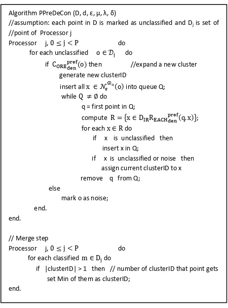
a) Sample database Algorithm PPreDeCon (D, d, ε, μ, λ, δ)
//assumption: each point in D is marked as unclassified and Dj is set of
//point of Processor j
Processor j, do for each unclassified do
if then //expand a new cluster generate new clusterID
insert all into queue Q; while do
q = first point in Q;
compute ;
for each do
if x
is unclassified then insert x in Q;
if x is unclassified or noise then assign current clusterID to x remove q from Q;
else
mark o as noise; end.
end.
// Merge step
Processor j, do for each classified do
if |clusterID| > 1 then // number of clusterID that point gets set Min of them as clusterID;
end. Algorithm PreDeCon(D, d, ε, μ, λ, δ)
// assumption: each point in D is marked as unclassified
for each unclassified do
if then //expand a new cluster
generate new clusterID
insert all ε into queue Q;
while do q = first point in Q;
compute ;
for each do
if x is unclassified then insert x in Q;
if x is unclassified or noise then assign current clusterID to x
remove q from Q; else // o is noise
mark o as noise; end.
[image:3.595.345.505.596.730.2]b) Clusters discovered by PPreDeCon
Fig 7: Checking accuracy with sample databases
So computing this vector needs checking the environment of the points in ε-neighborhood along each dimension which is done in . Therefore it takes for all points. According to definition 6, checking the preference weighted core point and expanding clusters, needs for all point in ε-neighborhood, evaluation of a weighted distance which can be
done in . Merge step is done in to compute minimum CID for all points. According to above
computations, A worst case time complexity ofthis algorithm
is . This yields a linear speedup against PreDeCon.
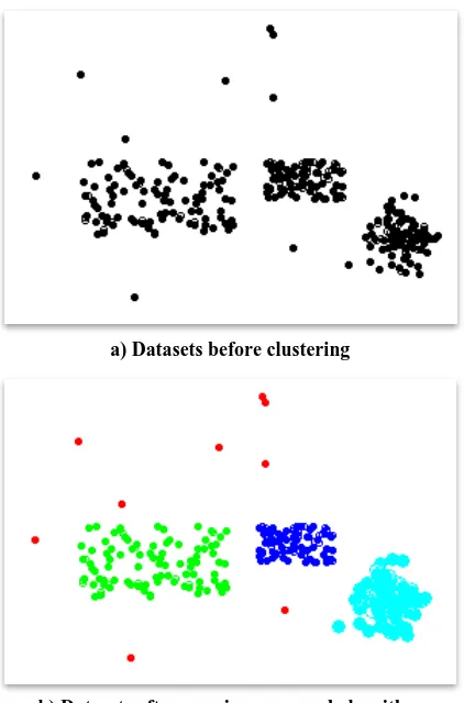
a) Datasets before clustering
[image:4.595.324.534.86.204.2]b) Datasets after running proposed algorithm
[image:4.595.329.554.307.476.2]Fig 8: Running proposed algorithm, PPreDeCon, in Dataset with noise
Table 1. run time of PreDeCon and PPreDeCon
Run time in seconds(P=2) Number of
points PPreDeCon
(proposed algorithm) PreDeCon
0.009 0.01
D1 = 50
0.021 0.03
D2 = 100
0.04 0.08
D3 = 250
0.054 0.09
D4 = 300
0.12 0.21
D5 = 500
5.
EXPERIMENTAL EVALUATION
In this section, accuracy and time-complexity of PPreDeCon are evaluated. For the evaluation, randomly generated data points within three clusters are used. It is depicted in fig 7. The dimension of the data sets is chosen as two. As it is shown in fig 7, the data points are randomly generated inside two rectangles and a circle.
Fig 9: Run time comparison between PreDeCon and PPreDeCon
In all experiments PPreDeCon discovered all the clusters and detected noises as good as PreDeCon. Lots of databases are used in these experiments which one of them is depicted in fig 8-a. This sample database contains three clusters with different shapes and sizes with additional noise. To show the result, each cluster is visualized by a different color. The result is depicted in fig 8-b. All clusters and noises discovered correctly.
Five 2-dimensional sample datasets are used to evaluate the run time of proposed algorithm.The experimental results are summarized in table 1. In these experiments the number of processors P is 2. The observation of the result shows that the run time of PPreDeCon is extremely lower than PreDeCon which is compared in fig 9.
6.
CONCLUSIONS
In this paper, a parallel clustering algorithm, PPreDeCon, is presented for mining large and high dimensional spatial databases. Lack of time can be solved by parallel computing. The parallel implementation uses shared memory model. The experiments showed that the actual clustering could be performed with good speed-up and good response time.
0.009 0.021
0.04 0.054
0.12
0.01
0.03
0.08
0.09
0.21
0 0.05 0.1 0.15 0.2 0.25 0.3 0.35
50 100 250 300 500
Ti
me
(se
co
n
d
s)
Number of Points
[image:4.595.62.273.375.695.2]As other advantages of this algorithm are accuracy and supporting high dimensional datasets and compared to other density-based clustering algorithms, it discovers the arbitrary shapes and is effective in noise detecting.
Future research may consider the following issues. Shared memory model is used for parallelism. However one may consider message passing model and also distributed memory. Concentration will be on density-based approaches. The parallelization of other spatial data mining methods may be considered in future. Computing times of all steps of the algorithm and focusing on reducing them maybe appropriate as future works.
7.
REFERENCES
[1] D. Joshi, A.K. Samal, and Leen-Kiat Soh,
"Density-based clustering of polygons," Computational
Intelligence and Data Mining: CIDM'09, IEEE , pp.171-178, 2009
[2] M. Ester, HP. Kriegel, J. Sander, X. Xu, “A density-based algorithm for discovering clusters in large spatial
databases with noise,” In Proc. 2nd Int. Conf. on
Knowledge Discovery and Data Mining: KDD, Vol.96, pp.226-231, 1996.
[3] J. Sander, M. Ester, HP Kriegel and X.Xu,
“Density-based clustering in spatial databases: The algorithm
GDBSCAN and its Applications,” Data Mining and
Knowledge Discovery, Vol.2, Iss.2, pp. 169-194, 1998.
[4] M. Ankerst, MM. Breunig, HP. Kriegel and J. Sander,
“OPTICS: ordering points to identify the clustering
structure,” ACM SIGMOD Record, Vol. 28, Iss.2, pp.
49-60, 1999.
[5] B. Zhou, D. W. Cheung and B. Kao, “A fast algorithm for density-based clustering in large database,”
Methodologies for Knowledge Discovery and Data Mining, Springer Berlin Heidelberg, Vol. 1574, pp. 338-349, 1999.
[6] Kim, Wooyoung, "Parallel clustering algorithms:
survey," CSC 8530 Parallel Algorithms, spring 2009.
[7] X. Xu, J. Jager, and HP. Kriegel, “A Fast Parallel
Clustering Algorithm for Large Spatial Databases,” High
Performance Data Mining, Springer, pp. 263 – 290, 2002.
[8] H. Meyerhenke, “PFDC: A Parallel Algorithm for Fast
Density-based Clustering in Large Spatial Databases,” In
Informatiktage 2002, Konradin Verlagsgruppe, pp. 48 – 52, 2003.
[9] C. Böhm, K. Railing and HP. Kriegel, “Density
connected clustering with local subspace preferences,”