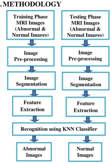
Detection and Classification of Brain Tumors

Automated testing of NFV orchestrators against carrier grade multi PoP scenarios using emulation based smoke testing Peuster et al EURASIP Journal on Wireless Communications and

LETTER Earth Planets Space, 63, 853?857, 2011 The resonant response of the ionosphere imaged after the 2011 off the Pacific coast of Tohoku Earthquake Lucie M Rolland1, Philippe

Bell, Gender, sex, & sexualities: Psychological perspectives.. Feminism

From the above exposure presented that the test results have also proved that with the use of Dakon’s game modification of children can manufacturer many objects,

Results of a oxidation of 2-(N-acetylamine)-3-(3,5-di- tert- butyl-4-hydroxyphenyl)-pro- pionic acid may by impotents in process research of products inhibitors of

Assume that we know the panel depth for both ascer- tainment experiments and that the discovery panel is part of the sample used to obtain the frequency spec- trum (as in case

To build a flexible hash function to satify different requirement, we propose construction AIMC that user can change the number of the step operations.. We just give

We find the threshold of the edge detection image and compare the pixels of the cover image with the threshold if it is greater than the threshold then we