Comparative study compact scheme for the case of shock tube problem

(1)

Comparative Study Compact Scheme for the Case of Shock Tube

Problem

MAHMOD ABD HAKIM MOHAMAD

Department of Mechanical Engineering

Centre for Diploma Studies

Universiti Tun Hussein Onn Malaysia

86400 Parit Raja, Batu Pahat Johor

MALAYSIA

MAHATHIR MOHAMAD

Department of Science and Mathematics

Faculty of Science,

Technology and Human Development

Universiti Tun Hussein Onn Malaysia

86400 Parit Raja, Batu Pahat Johor

MALAYSIA

Abstract: In this work, a high-order compact upwind scheme is developed for solving one-dimensional Euler equation. A detailed investigation was conducted to assess the performance of the basic third-order compact central discretization schemes. From this observation, discretization of the convective flux terms of the Euler equation is based on a hybrid flux-vector splitting, known as the advection upstream splitting method (AUSM) scheme which combines the accuracy of flux-difference splitting and the robustness of flux-vector splitting. In one-dimensional problem for the first order schemes, an explicit method is adopted by using time integration method. In addition to that, development and modification of source code for the one-dimensional flow is validated with two test cases namely, unsteady shock tube and quasi-one-dimensional supersonic-subsonic nozzle flow were using as a comparative study. Further analysis had also been done in comparing the characteristic of AUSM scheme against experimental results, obtained from previous works and also comparative analysis with computational results generated by van Leer, KFVS and AUSMPW schemes. Furthermore, there is a remarkable improvement with the extension of the AUSM scheme from first-order to third-first-order accuracy in terms of shocks, contact discontinuities and rarefaction waves.

Key-Words: High-order compact schemes, finite difference methods, flux-difference splitting, flux-vector splitting, Euler equations, One-dimensional.

1 Introduction

The most general approach to the analysis of compressible inviscid flows must choose to the Euler equations. These compressible inviscid flows including rotational, non-isentropic, non-heat-conducting and non-viscous flows effects require simultaneous solutions of continuity, momentum and energy equations. The numerical solution of the Euler equations is determined while through the space or time to obtain a final numerical description of the physically and geometrically complex flow of engineering relevance. The computed results complement experimental and theoretical techniques

(2)

simple and robust for capturing of intense shocks and rarefaction waves. However, while FVS is based on scalar calculations and FDS is based on matrix calculations. [5] have proposed AUSM (Advection Upstream Splitting Method) that has the accuracy of FDS schemes and the robustness and efficiency of FVS schemes. In this method, the inviscid flux at a cell interface is split into a convective contribution, upwinded in the direction of the flow and a pressure contribution which is upwinded based on acoustic considerations. The direction of the flow is determined by the sign of a Mach number defined by combining information from both the left and right states about the cell interface.

In this work the computational code using AUSM scheme was used to develop a one-dimensional Euler solver by using high-order compact finite-difference techniques for compressible flows. The validation was used up to

the 3rd-order against experimental and comparison

of computational results due to van Leer, KFVS and AUSMPW schemes. Due to the efficiency of the scheme as observed by other researchers namely

[6,7,8], [9],[10], [11], [12], [13], [14] [15,16,17],

[18] and [19]. Besides that, the characteristic of the numerical method was not compared completely with the other schemes. The test problems considered contain various types of discontinuities, such as shock waves, rarefaction waves and contact surfaces. In the absence of available CFD code, a comprehensive validation of code is required and the AUSM scheme has yet to be validated for a wide range of cases. For this reason, a systematic approach has to be adopted to examine the AUSM scheme before the method can be applied to a more complicated and complex compressible flow

problems. Further analysis had also been done in

comparing the characteristic of AUSM scheme against experimental results, obtained from previous works and also comparative analysis with computational results generated due to van Leer, KFVS and AUSMPW schemes.

2 The Basic Discretization Method

2.1 Spatial Discretization and Numerical

Fluxes

The model equation for nonlinear scalar conservation law in one-dimensional space can be written as [1,2]

(

)

=

0 ∂

∂

+

∂

x

u

f

t

u

(1)

with the subject to the given initial condition [1,2]

u

(

x

,

0 )

=

u

0

(

x

)

(2)

where x

u f

∂ ∂ ( )

is some vector-valued function of u.

Equation (2), is specialised to

) 0 ( ) 0 , (

> ≡

< ≡

x u x u

R

L ₍₃₎

Equation (1) can be written in split flux form as [4]

( ) ( )=0

∂ ∂ + ∂ ∂ + ∂

∂ + −

x u f x

u f t u

(4)

where

f

(

u

)

=

f

+

(

u

)

+

f

−

(

u

).

This flux vector

splitting has been introduced by [3]. The split fluxes

)

(

u

f

+ and

f

−

(

u

)

are also homogeneous functions

of degree one in u [20]. Conservative

semidiscretization of equation (4) can be written as [4]

+(ˆ 1/2 − ˆ 1/2)/∆ =0

∂ ∂

−

+ f x

f t u

i i

i

(5)

where

f

ˆ

_i₊₁_/₂ and

f

ˆ

_i₋₁_/₂ is known as the numerical flux function.

First-order upwind approximation to the numerical flux is given by [4]

− + − −

− + + +

−

=

+

=

i i i

f

1 2 / 1

1 2

/ 1

ˆ

(6)

Following [4], a high-order numerical flux can be

obtained as follows. The numerical flux

f

ˆ

_i₊₁_/₂ is

decomposed into positive and negative parts,

+ +1/2

ˆ

i

f

and

f

ˆ

_i₊−₁_/₂ such that

− + +

+

+1/2

=

ˆ

1/2

+

ˆ

1/2

ˆ

i i

i

f

(7)

(3)

F

_i

=

f

ˆ

_i₊₁_/₂

−

f

ˆ

_i₋₁_/₂ (8)

where

F

_i

/

∆

x

is a high-order approximation to the

derivative

x

u

f

_i

∂



(

)

, to be determined by a

high-order compact scheme.

[21] has presented a third-order approximation to a first derivative by an upwind based compact relation as         _ _ 1 1 1

1 60 15 52.5 15 37.5

75 .

18 Fi± + Fi + Fi =± fi± fi fi (9)

Equation (9) can be written for the interior points

2

=

i toi=N −1. For the boundary points i =1

and

i

=

N

, the following second order explicit

relations are used

    3 2 1

1 1.5f 2f 0.5f

F = − + − (10)

 

2

1 0.5

2 5 .

1 − ₋ + ₋

= _N _N _N

N f f f

F (11)

Plugging equation (8) in equation (9) yields the following relations for the interior points

2

=

i toi=N −1.

+ + + + + + + +

− + i + i = i + i

i f f f f

fˆ 60ˆ 11.25ˆ 37.5 52.5 75

.

18 1/2 1/2 3/2 1 (12)

− − + − + − + −

− + i + i = i + i

i f f f f

fˆ 60ˆ 18.75ˆ 52.5 37.5 25

.

11 1/2 1/2 3/2 1 (13)

With

F

₁ and FN evaluated explicitly, two sets of

(N - 1) equations are to be inverted for the split

numerical fluxes

f

ˆ

i+1/2. Before using these fluxes it

is necessary to limit their values and this is achieved by defining the differences

− + − + − + + + + + +

−

=

−

=

2 / 1 1 2 / 1 2 / 1 2 / 1

ˆ

i i i i i i

f

d

f

d

(14)

and limiting by the limiter

) , ˆ mod( min ˆ ) , ˆ mod( min ˆ 2 / 1 ) ( 2 / 1 2 / 1 ) ( 2 / 1 − − + − + + + + + + = = D f d f d D f d f d i m i i m i (15)

The third-order TVD flux differences of [22] may be used here

)) , mod( min 2 ) , mod( (min 6 1 1

1 + + + + + +−

+ − + +₌ ₊ i i i

i f f f

f

D δ λδ δ λδ (16)

)) , mod( min 2 ) , mod( (min 6 1 1 1 − + + − + − + − + + −₌ ₊ i i i

i f f f

f

D δ λδ δ λδ (17)

where 1≤

λ

≤4.

The limited numerical fluxes are then calculated from ) ( 2 / 1 1 ) ( 2 / 1 ) ( 2 / 1 ) ( 2 / 1

ˆ

m i i m i m i i m i

f

d

f

d

f

− + − + − + + + + + +

−

=

+

=

(18) and

1(/2)

) ( 2 / 1 ) ( 2 /

1

ˆ

m

i m i m

i

f

₊

=

+₊

+

−₊ (19)

The min mod function can be defined as

     < > < > < = 0 ) ( 0 0 ) ( , 0 ) ( , ) , mod( min ab if ab a b if b ab b a if a b

a (20)

3 Euler Equations and Flux Splitting

Scheme

The one-dimensional Euler equation may be written as

=

0 ∂

∂

+

∂

x

E

t

Q

(21) where

,













=

e

u

Q

ρ

          + = uH p u u E

ρ

2

and ρ, u, p, e and H are the density, velocity,

pressure, total energy, and total enthalpy

respectively. The total enthalpy H, is related to the

other quantities by the relation

ρ

p

e

H

=

+

(22)

and for a perfect gas

2

1 )

1 (

u

p

e

+

−

=

γ

(4)

where

γ

is the ratio of specific heat and takes the value of 1.4 for air.

The extension of the scalar high order numerical fluxes developed above to Euler equations is straightforward. The AUSM flux splitting technique used here is detailed in references [5, 21]. Once the

split fluxes E_i±are obtained then the method

described above is used to obtain the higher order numerical fluxes. Equation (18) is, thus, written in a semidiscretized form as

L(Q)

t

Q ₌

∂ ∂

(24)

where

L

Q

E

x

m i m

i

−

∆

−

=

(

+ −

)

/

)

(

) (

2 / 1 ^ ) (

2 / 1 ^

(25)

Using the method-of-lines [4], the systems of equations (21) are integrated by a multistage TVD Runge-Kutta scheme [22].

4 Boundary Conditions

For the shock tube problem considered in this paper, a short time span for unsteady flow is considered such that the waves will not reach the end walls and so conditions at these boundaries are held fixed. Meanwhile, for the supersonic-subsonic nozzle problem, one type of boundary conditions i.e. inflow/outflow is encountered. At the supersonic inflow, values of velocity, density and pressure are specified while at the subsonic outflow the velocity is specified and the density and pressure are extrapolated from the interior.

5 Results and Discussion

In this study, two problems are considered as the shock tube problems such as unsteady shock tube and quasi one-dimensional flow in a divergent nozzle were using as a comparative study. In addition, the computed results were compared with available exact solutions, and numerical results from other schemes, such as AUSM scheme, AUSMPW scheme, van Leer’s scheme and KFVS scheme. Results are also shown with first-order accurate upwind space discretization compared with up to third-order compact scheme.

The first problem considered is the unsteady shock tube problem. This problem is an interesting

test case to assess the ability of a compressible code to capture shocks and contact discontinuities and to produce exact profiles in the rarefaction wave. The

problem spatial domain is 0 ≤ x ≤ 1. The initial

solution of the problem consists of two uniform states, termed as left and right states, separated by a

discontinuity at x = 0.5. As in the first problem,

results are obtained using first-order and third-order upwind schemes with the AUSM scheme, van Leer’s scheme and KFVS scheme. The number of mesh points used is 101 and CFL = 0.2. The initial conditions of the left and right states are

(ρL, uL, pL) = (1, 0, 1)

(ρR, uR, pR) = (0.125, 0, 0.1)

The wave pattern of this problem consists of a rightward moving shock wave, a leftward moving rarefaction wave and a contact discontinuity separating the shock and rarefaction waves and moving rightward. Fig. 1 shows results obtained by the first order and third-order accurate schemes for the distribution of pressure, density and velocity

along the tube at time, t = 0.2 units, in comparison

with the exact solution. From the numerical results

of the 1st-order schemes for this particular problem,

two observations can be made: first, the solutions produced are non-oscillatory and second, shock

smearing is present in both 1st-order schemes with

the degree of shock smearing more apparent in the KFVS scheme in comparison with the AUSM scheme. In addition, it is shows that in the density profile the contact discontinuity is narrowly visible and in the velocity profile there is a minor overshoot at the right corner of the expansion wave. Meanwhile, the transition of the shock wave in the velocity profile occupies eleven to twelve zones.

From the numerical result of up to 3rd-order

schemes, it is shows that the AUSM scheme is able to produce non-oscillatory and crisp shock transition, which can hardly be obtained from the KFVS and van Leer schemes. This is true as the results produced by the KFVS scheme are more diffusive in comparison with the AUSM scheme, while the van Leer scheme generated a small jump around the contact discontinuity in the velocity distribution. In addition, it is shows that in the density profile the contact discontinuity is narrowly visible especially at AUSM scheme compare to the other schemes. Meanwhile, the transition of the shock wave in the velocity profile occupies four to six zones. Beside these findings, it is also observed

that the 3rd-order AUSM scheme is able to produce

(5)

KFVS and 5th-order compact upwind van Leer schemes.

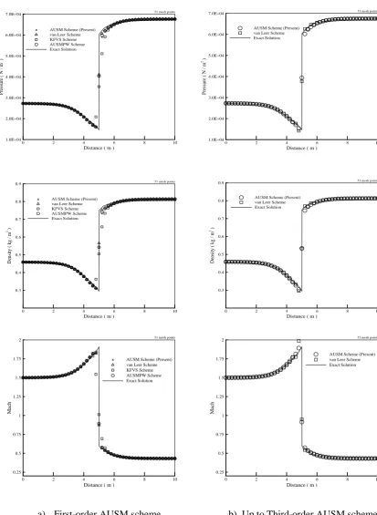
The second problem considered is a quasi one-dimensional supersonic-subsonic flow in a divergent

nozzle. The nozzle cross-section S(x) varies

according to

S(x) = 1.398 + 0.347 tanh

(

0 .

8 (

x

−

4 )

)

; 0 ≤x≤ 10

The inflow and outflow conditions are

(ρ1, u1, p1) = (0.459, 432.5, 0.2724 x 10

5

)

(ρN, uN, pN) = (0.811, 146.94, 0.673 x 10

5

)

These conditions correspond to a normal shock at

x = 5 with supersonic flow at the inlet Mach number

M1 = 1.5 and subsonic flow at the outlet Mach

number MN = 0.431. Calculation are performed with

a time step, ∆t corresponding to

Courant-Friedrichs-Lewy, CFL number = 1. The number of points used to solve this problem is N = 51. The integration in time is continued until steady state is reached. The solution is assumed to converge when the absolute

value of the residual in pressure pn+1– pn≤ 0.1.

Fig. 2 shows first-order and third-order upwind results for the distribution of pressure, density and Mach number along the flow in comparison with the exact solution. The numerical solution shows that

the 1st-order AUSMPW scheme is able to produce

solutions that outweigh other numerical solutions schemes. These are justified by the over-diffusivity of the KFVS and AUSM schemes around the region of the shock after the shock as clearly. While the numerical solutions of the AUSMPW and van Leer schemes are observed to have almost similar performance, where the van Leer scheme is able to produce a slightly better shock resolution for the pressure distribution, the AUSMPW scheme leads the shock resolution for the density and Mach number distributions. In Fig. 2, it also shows that the

numerical solutions computed by a 5th-order

compact upwind van Leer scheme [15] are also used

to compare with the 3rd-order AUSM scheme and it

revealed that the degrees of post-shock oscillations are more severe within the van Leer scheme in

comparison to the AUSM scheme.

6 Conclusion

A third-order compact upwind method based on the flux-vector splitting approach was developed for high speed inviscid flows. A new flux limiting procedure, different from those used in similar

approaches, was introduced for resolving shock waves and other types of discontinuities without spurious oscillations. The scheme is tested by performing calculations for a compressible flows shock tube cases namely unsteady shock tube and quasi one-dimensional flow in a divergent nozzle.

Results are also presented to validate up to the 3rd

-order AUSM scheme against experimental and comparison of computational results due to van Leer, KFVS and AUSMPW schemes. From this result, it was found that by using the AUSM scheme

from 1st-order to 3rd-order accuracy especially in

unsteady shock tube and steady-state numerical solutions of the divergent nozzle, the improvement of shock capturing properties such as the accuracy of shocks, contact discontinuities and rarefaction waves were achieved.

7 Acknowledgments

The present author acknowledges the members of our research study especially to Dr Mahmood Khalid Mawlood and also Dr Bambang Basuno for his helpful discussions, advice, encouragement and support throughout this study.

References:

[1] P. L. Roe, Approximate Riemann Solvers,

Parameter Vectors, and Difference Schemes,

Journal of Computational Physics, Vol. 43, 1981, pp. 357-372.

[2] Steger, J. L. and Warming, R. F., Flux Vector

Splitting of the Inviscid Gas Dynamic Equations with Application to Finite Difference

Methods, Journal of Computational Physics,

Vol. 40, 1981, pp. 263-293.

[3] Van Leer, B., Flux Vector Splitting for the

Euler Equation, Lecture Notes in Physics, Vol.

170, 1982, pp. 507-512.

[4] Ravichandran, K. S., High Order KFVS

Algorithms Using Compact Upwind Difference

Operators, Journal of Computational Physics,

Vol. 130, 1997, pp. 161-173.

[5] Liou, M. S. and Steffen, C. J. Jr., A New Flux

Splitting Scheme, Journal of Computational

Physics, Vol. 107, 1993, pp. 23-39.

[6] Liou, M.-S. and C. J. Steffen, Jr., Development

of a New Flux Splitting Scheme, Center for

Modeling of Turbulence and Transition (CMOTT), 1990, pp. 144-145.

[7] Liou, M.-S., On a New Class of Flux Splittings,

(6)

[8] Liou, M.-S., A Sequal to AUSM: AUSM+,

[9] Radespiel, R. and Kroll, N., Accurate Flux

Vector Splitting for Shocks and Shear Layers,

[10]Billet, G. and Louedin, O., Adaptive Limiters

for Improving the Accuracy of the MUSCL

Approach for Unsteady Flows, Journal of

Computational Physics, Vol. 170, 2001, pp. 161-183.

[11]Mary, I. and Sagaut, P., Large Eddy Simulation

of Flow Around An Airfoil Near Stall, AIAA

Journal, Vol. 40, 2002, pp. 1139 – 1145.

[12]Evje, S. and Fjelde, K. K., On A Rough AUSM

Scheme for One-Dimensional Two-Phase

Model, Computers and Fluids, Vol. 32, 2003,

pp. 1479-1530.

[13]Manoha, E., Redonnet, S. Terracol, M., and

Guenanff, G., Numerical Simulation of

Aerodynamics Noise, ECCOMAS, 24 – 28 July

2004.

[14]Wada, K. and Koda, J., Instabilities of Spiral

Shock – I. Onset of Wiggle Instability and Its Mechanism. Monthly Notices of the Royal Astronomical Society, Vol. 349, No. 11, 2004, pp. 270-280.

[15]Mawlood, M. K., Asrar, W., Omar, A. A. and

Basri, S., A Higher-Order Shock Capturing

Scheme for Inviscid Flows, Proceedings, 2nd

World Engineering Congress, Sarawak, Malaysia, 2002, pp. 383-388.

[16]Mawlood, M. K., Asrar, W., Omar, A.A. and

Basri, S., A High-Resolution Compact Upwind

Algorithm for Inviscid Flows, 41st Aerospace

Sciences Meeting and Exhibit Conference, AIAA, 2003-0076, USA, 2003.

[17]Mawlood, M. K., Basri, S., Asrar, W., Omar,

A. A., Mokhtar, A. S. and Ahmad M. M. H. M., Solution of Navier-Stokes Equations By Fourth-Order Compact Schemes and AUSM

Flux Splitting, International Journal of

Numerical Methods for Heat & Fluid Flow, Vol. 16, No. 1, 2006, pp. 107-120.

[18]Zha, G. C. and Hu, Z., Calculation of Transonic

Internal Flows Using an Efficient

High-Resolution Upwind Scheme, AIAA Journal,

Vol. 42, No. 2, 2004, pp. 205 – 214.

[19]A. Chaudhuri, C. Guha and T. K. Dutta,

Application of AUSM And AUSM+ In Inviscid

Flow, CHEMCON-05, New Delhi, Session:

Computational Fluid Dynamics, 2005, pp. 1-8.

[20]Hirsch, C., Numerical Computation of Internal

and External Flows. Vol. 2: Computational

Methods for Inviscid and Viscous Flows. John

Wiley and Sons, UK, 1990.

[21]Zhong, X., High-Order Finite-Difference

Schemes for Numerical Simulation of Hypersonic Boundary-Layer Transition,

[22]Yee, H. C., Upwind and Symmetric Shock

(7)

Distance ( m )

P

re

ss

ur

e

(

N

/m

2)

0 0.2 0.4 0.6 0.8 1

AUSM Scheme (1st

) (Present) KFVS Scheme (1st

) Exact Solution

101 mesh points

Distance ( m )

P

re

ss

ur

e

(

N

/m

2)

0 0.2 0.4 0.6 0.8 1

0 0.2 0.4 0.6 0.8

1 AUSM Scheme (3rd

) (Present) KFVS Scheme (3rd

) van Leer Scheme (5th

) Exact Solution

101 mesh points

Distance ( m )

D

en

si

ty

(

kg

/m

3)

0 0.2 0.4 0.6 0.8 1

AUSM Scheme (1st

) (Present) KFVS Scheme (1st₎

Exact Solution

101 mesh points

Distance ( m )

D

en

si

ty

(

kg

/m

3)

0 0.2 0.4 0.6 0.8 1

0 0.2 0.4 0.6 0.8

1 AUSM Scheme (3rd_{) (Present)}

KFVS Scheme (3rd₎

van Leer Scheme (5th

) Exact Solution

101 mesh points

Distance ( m )

V

el

oc

it

y

(

m

/s

)

0 0.2 0.4 0.6 0.8 1

AUSM Scheme (1st_{) (Present)}

KFVS Scheme (1st₎

Exact Solution

101 mesh points

Distance ( m )

V

el

oc

ity

(

m

/s

)

0 0.2 0.4 0.6 0.8 1

AUSM Scheme (3rd_{) (Present)}

KFVS Scheme (3rd₎

van Leer Scheme (5th₎

Exact Solution

101 mesh points

a) First-order AUSM scheme b) Up to Third-order AUSM scheme

(8)

x x x x x x x x x x x x x x_{x x} xx_x

x x

x_x x

x xx

xx x

x x xx x x x x x x x x x x x x x x x

Distance ( m )

P

re

ss

u

re

(

N

/

m

2)

0 2 4 6 8 10

1.0E+04 2.0E+04 3.0E+04 4.0E+04 5.0E+04 6.0E+04 7.0E+04

AUSM Scheme (Present) van Leer Scheme KFVS Scheme AUSMPW Scheme Exact Solution

x

51 mesh points

Distance ( m )

P

re

ss

u

re

(

N

/

m

2)

0 2 4 6 8 10

1.0E+04 2.0E+04 3.0E+04 4.0E+04 5.0E+04 6.0E+04 7.0E+04

AUSM Scheme (Present) van Leer Scheme Exact Solution

51 mesh points

x x x x x x x x x x x x x x_{x x} xx

x x

x xx

x xx x x

x x x x x x x x x x x x x x x x x

Distance ( m )

D

en

si

ty

(

kg

/

m

3)

0 2 4 6 8 10

0.3 0.4 0.5 0.6 0.7 0.8 0.9

x

51 mesh points

Distance ( m )

D

en

si

ty

(

kg

/

m

3)

0 2 4 6 8 10

0.3 0.4 0.5 0.6 0.7 0.8 0.9

51 mesh points

x x x x x x x x x x x x xx x x x x

xx xx

x x x

x

x x

x x

x x x x x x x x xx x x x x x x x x x x x

Distance ( m )

M

ac

h

0 2 4 6 8 10

0.25 0.5 0.75 1 1.25 1.5 1.75 2

x

51 mesh points

Distance ( m )

M

ac

h

0 2 4 6 8 10

0.25 0.5 0.75 1 1.25 1.5 1.75 2

51 mesh points

[image:8.595.87.501.93.659.2]

a) First-order AUSM scheme b) Up to Third-order AUSM scheme

Comparative study compact scheme for the case of shock tube problem