An Improvement of LEACH Algorithm Based on TinyOS for Wireless Sensor Network

2016 6th International Conference on Information Technology for Manufacturing Systems (ITMS 2016) ISBN: 978-1-60595-353-3

1 INTRODUCTION

Wireless sensor network (WSN) combine the sensor technology, embedded technology and wireless communications technology. It consists of a large number of micro sensor nodes, and is widely used for a various applications, such as environmental monitoring, disaster prevention and traffic control.

Due to sensor nodes’ battery energy, computing and storage capacity is limited, the operating system they required should be less energy consumption and can adapt to all kinds of application environment. TinyOS operating system is an event-based system, and it uses the component hierarchy. At present most of the WSN research projects use the TinyOS operating system. TinyOS has become a standard platform in the WSN research field.

The function of WSN routing protocol is to search for the path from the source node to the destination node, and transmit the data along with the searching path. Routing protocol is the kernel of WSN that determines the operation efficiency and implementation performance. The WSN routing protocol algorithm should be designed with the goal of reducing the network energy consumption as much as possible.

LEACH (Low Energy Adaptive Clustering Hierarchy) is the most typical clustering routing protocol. It has the feature of low energy consumption and self-adaption. Each round of LEACH algorithm is made up of two stages as cluster establishment and data transmission. In the stage of cluster establishment, each sensor node

generates a random number between 0~1. If this generated number is smaller than the thresholdTn,

this node will be selected as the cluster head. The cluster nodes that are not cluster heads will choose to join their nearest cluster head to form a cluster in line with the broadcast they have received. The equation of Tn is:

1 [ m o d (1 / )] 0

n

P

n G

P r P

T

n G

 _∈

 _{− ×}

=_

 ∉

 (1)

Where P = the expected percentage of cluster heads’ number in the total number of all nodes; r = the current round number; each 1/P round is a period; and G = the node set of the nodes that are not selected as cluster heads in the latest period.

In the stage of data transmission, the cluster member nodes send the collected data to their cluster head; the cluster head will then conduct the data fusion process and send the processed data to the base station in way of single hop.

However, many deficiencies exist in LEACH algorithm, and they can be concluded as following:

a) LEACH algorithm chooses cluster heads in a random way, which cannot ensure even distribution of the clusters. As the cluster heads are distributed unevenly, their energy consumption could be quite different, and this will surely shorten the lifetime of the network.

b) In LEACH algorithm, the cluster head node uses single hop to communicate with the base station, which will rapidly consume its energy when the head node is some distance from the base station.

An Improvement of LEACH Algorithm Based on TinyOS for

Wireless Sensor Network

M. Zhu & M.D. Liu

College of Information Science and engineering, East China University of Science and Technology, Shanghai 200237, China

Focusing on the above disadvantages of LEACH, an energy-saving and highly-efficient multi-hop routing algorithm is proposed, and it is called LEACH-EEMH (Energy Efficient Multi-hop).

2 LEACH-EEMH ALGORITHM

2.1 Energy consumption model

The energy model of LEACH-EEMH algorithm is the same as LEACH; it is a first-order wireless energy consumption model.

According to this model, when the node sends kbits of data to a certain place with a distance of d, the energy consumption of this process can be calculated as following:

2 0 4 0 ( , ) elec fs tx elec mp

kE k d d d

E k d

kE k d d d

ε

ε

 + <

 =_

+ ≥

 (2)

Where Eelec = the energy consumption required by

sending or receiving unit bit data; ε_fs = the power

amplification loss constants in free-space model; and

ε_mp

= multi-channel attenuation mode. When the transmission distance is smaller than threshold d0,

the power amplification loss uses the free-space model; when the transmission distance is larger than the threshold d0, the multi-channel attenuation model

should be used. Apparently, the latter consumes much more energy than the former.

The energy consumed when the sensor node receives k bits data can be calculated as following:

( , )

rx elec

E k d =kE

(3) The energy consumed when the sensor node fuses

k bits data can be calculated as following:

( , )

fusion DA

E k d =kE

(4) Where EDA = the energy consumed when the node

fusing unit bit data.

2.2 Calculation of the optimal cluster heads separation distance

The optimal separation distance between cluster head nodes is calculated according to the optimal cluster heads number. Therefore, the first step is to calculate the optimal number of cluster head nodes.

Assuming that there are n _{nodes distributed}

randomly in a M × M monitoring region; In this

condition, if there are k number of clusters, and then

there will be an average of n/k _{nodes in each cluster.}

The energy consumption of cluster head includes receiving the data collected by member nodes, fusing the data in cluster, and transferring the processed data to the base station. Since the head node is some distance from the base station, its energy consumption can be calculated in line with the

multi-channel attenuation model. The energy consumption of each cluster head node is:

4

( 1)

ch elec DA mp toBS

n n

E E l E l ld

k k

ε

= − + +

(5) Where l= the size of the data packet; dtoBS = the

distance between the head node and the base station. The energy consumption of the member nodes is mainly caused when they send the collected data to the cluster head. If the distance between the head node and its member nodes is relatively small, the free-space model can be used, and the energy consumption of each member node will be:

(

)

cm elec fs toCH

E =l E +ε d

(6) Where dtoCH = the distance between the member

node and the cluster head.

The cluster can be treated as a circular region taking the cluster as its center, because the member nodes choose their cluster heads based on the distance between them and the cluster head. The average cover area of each cluster is M/k; the square

expected value of the distance between the cluster head and its member nodes is:

(

)

(

)

2 2 2 3 0 0 ( , ) ( , ) 2 ch toch M N ch

E d x y x y dxdy

M

r r drd r drd

N π

π ρ

ρ θ θ ρ θ

π

= +

= = =

∫∫

∫∫

∫ ∫

Hence, the energy consumption of the member node can be expressed as:

2

2

cm elec fs

M

E lE l

k

ε π

= + (8)

The energy consumption of each cluster is:

( 1)

cluster ch cm

n

E E E

k

= + −

(9) Consequently, the energy consumption of the entire network can be written as:

2 4

( )

2

fs

total cluster elec DA mp toBS

n M

E kE l nE nE k D

k ε ε π = = + + + (10)

Where DtoBS = the distance between the base

station and the network area center.

Set the first-order derivative to be 0. Then, the k

value that leads to the smallest Etotal can be

calculated through the following equation:

2 2 fs opt mp toBS n M k D ε π ε

= (11)

The death of nodes exists continuously during the entire running process of the network as their energy are used up. Therefore, kopt value is variable.

It is known that the monitoring region is a square with an area of M × M, which should be fully

covered by kopt clusters. Hence, the distance between

clusters should be evenly distributed. As shown in Figure 1, R is the radius of the circle taking the

cluster head as its center; √_{2R is the side length of}

the circle’s inscribed square. The entire M×M

monitoring region is covered by kopt small squares.

Then, an equation can be established as following:

(

)

opt

k × R =M×M (12)

The radius of the cluster R is:

2 opt

R=M K (13)

Then, the smallest separation distance between cluster heads will be:

2 opt

D= R=M K (14)

According to equation (14), D changes along with kopt. In LEACH-EEMH algorithm, D value will be

recalculated in each period (1/P round) of the base

station, and then be broadcast to the entire network.

Figure 1. Reasonable network topology structure. 2.3 Process of LEACH-EEMH algorithm

Each round of LEACH-EEMH consists of three stages as the establishment of cluster, the formation of multi-hop paths between clusters, and data transmission.

2.3.1 Establishment of the cluster

This stage includes two parts: the first-round cluster establishment of a period; the non-first-round cluster establishment.

a) The first-round cluster establishment of a period:

Before the election of cluster heads, each node should arrange a time for countdown in accordance with its energy level. Nodes with large amount of energy will have shorter countdown time; nodes with smaller amount of energy should arrange longer time.

When the election of cluster heads starts, the whole network enters the countdown process. The node with the largest amount of energy will be the first to end its countdown and be selected as the first cluster head. Then, this node will broadcast this message in the communication radius of D. Then it

lengthens this communication radius to send a cluster head message to the base station.

Within the arranged time, if one of the nodes receives the broadcast message from the cluster head, its countdown process will be ended immediately and this node will give up to be a cluster head. For the nodes that haven’t receive any cluster head’s broadcast during the entire countdown process, they will announce themselves as cluster heads as soon as the countdown process ends.

If broadcast messages of cluster heads the base station receives indicates that the number of cluster heads has reached its optimal, the election of cluster heads will be ended.

When the election process ends, cluster nodes will enlarge the communication radius to broadcast the cluster head message. The non-cluster head chooses its nearest head node as its cluster head according to the strength of the signal. Then, it should send a request to this cluster to join it.

b) Non-first-round cluster establishment of a period:

In this stage, there is no need for reassembling in the entire network. Cluster heads for the current round are allocated by the heads of the previous round. In the last stage of the steady data transmission process, cluster heads of the previous round choose the nodes that have the largest remaining energy as cluster heads for the next round. These selected new cluster heads broadcast this message; non cluster head nodes join the cluster.

2.3.2 Establishment of multi-hop routing between clusters

Each cluster head maintains a route table Troute. This

table is built in line with the messages receiving from cluster heads. When the cluster head i receives

the broadcast of cluster head j, the separation

distance dtoBS between the base station and these two

cluster heads will be calculated and compared. If the

dtoBS of j is smaller than the dtoBS of i, the cluster

head j should join i’s route table Troute.

In the following two cases, the cluster head node will chose the node of its next hop.

If cluster head i’s dtoBS is not larger than d0 or its

Troute is empty, then, the base station will be chosen

as the node for the next hop. Otherwise, cluster head

i should choose the nearest node from its Troute as the

next hop.

2.3.3 Data transmission

3 IMPLEMENTATION OF LEACH-EEMH ON TINYOS

3.1 Overall framework

In this paper, TinyOS 2.1 operation system and nesC language are used to implement LEACH-EEMH protocol.

The objective function is divided into upper layer functions and lower layer functions on TinyOS. The modules are connected by interfaces. Interfaces are bidirectional. Upper layer modules can use the functions of the lower layer modules via interfaces; lower layer modules trigger events to the upper layer modules. Configuration represents the connection

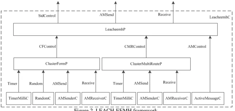
relation between modules. Figure 2 shows the overall framework of LEACH-EEMH protocol. The solid line boxes stand for modules; the dotted line boxes stand for configuration; arrows stand for interfaces. Above the arrows there are upper layer modules; below the arrows are lower layer modules.

LEACH-EEMH protocol adopts the model of single configuration but multiple modules. The whole protocol is implemented within the configuration—LeacheemhC. LeacheemhC components provide the upper layer with interfaces related to data transmission, such as StdControl, AMSend and Receive interface.

Figure 2. LEACH-EEMH framework. 3.2 Main function modules

LEACH-EEMH protocol is mainly made up of three modules as LeacheemhP, ClusterFormP and ClusterMultiRouteP. LeacheemhP is the administrator of the other two modules, offer open functional interface for the outside. ClusterFormP is the cluster establishment module, and ClusterMultiRouteP is the inter-cluster multi-hop routing module.

3.2.1 LeacheemhP module

LeacheemhP is the key processing module of LEACH-EEMH protocol. LeacheemhP controls the start and close of the wireless communication module by calling the AMControl interface; it controls the ClusterFormP to finish the establishment of the cluster by calling the CFControl interface; it calls the CMRControl interface to control the ClusterMultiRouteP module to build the inter-cluster multi-hop routing.

LeacheemhP module provides the upper layer with StdControl, AMSend and Receive interface. StdControl is a standard control interface that can control the start and close of the routing layer functions. AMSend is a message sending interface. The essence of AMSend is to reach the target via the multi-hop transmission of the routing layer. The

destination address of the LEACH-EEMH protocol is the base station. Receive is the interface that receives messages. When the base station receive the message package, the event of Receive interface will be triggered.

3.2.2 ClusterformP module

ClusterFormP is the cluster establishment module which is responsible for the election of cluster heads, the formation and maintenance of the cluster. It provides the upper layer with CFControl interface, which can be applied to control the start and close of cluster establishment process.

ClusterFormP calls AMSend interface and Receive interface to realize the sending and receiving of the inner-cluster routing and the data packet. It calls TimerMilliC’s Timer interface to finish a series of timer-related operations. It calls RandomC’s Random interface to obtain the random value required by the cluster head election.

3.2.3 Cluster multi route P module

routing establishment, and the acquisition of routing information.

ClusterMultiRouteP module calls AMS end interface and receive interface to send inter-cluster routing or receive data packet. It also invokes TimerMilliC’s Timer interface to complete a series of timer-related operations.

4 SIMULATION EXPERIMENT

4.1 Simulation parameter settings

In this paper, the built-in simulation tool TOSSIM (TinyOS simulator) is applied to simulate LEACH-EEMH algorithm. TOSSIM can support large scale of network simulation.

Set the coordinates of the base station to be (50, 175); 100 nodes are randomly distributed in a 100m×100m monitoring area. The detailed simulation parameters are listed in Table 1.

Table 1. Simulation parameters.

Parameter Parameter Value

Node’s Initial Energy 2J

Eelec 50nJ/bit

ε_{fs 10pJ/bit/m}2

ε_{mp 0.0013pJ/bit/m}4

EDA 5nJ/bit

d0 87m

Length of Data Packet 4000bits

4.2 Simulation results and analysis

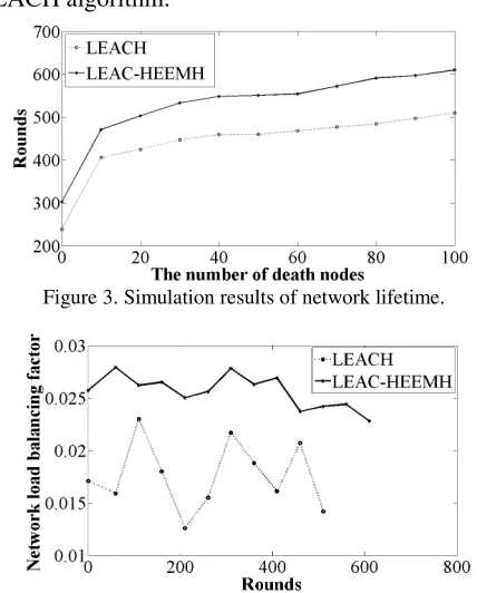
Network lifetime and load balancing degree are applied as two performance evaluation indexes to make comparisons between LEACH-EEMH and LEACH algorithm.

Figure 3. Simulation results of network lifetime.

Figure 4. Simulation results of network load balancing factor.

As shown in Figure 3, the node that dies first in LEACH algorithm has worked for 240 rounds, while the node dies last has worked for 510 rounds. In LEACH-EEMH algorithm, these two values are 300 rounds and 610 rounds, respectively. It’s clear that the network lifetime of LEACH-EEMH algorithm is much longer than that of LEACH. Main reasons for this are as following:

a) LEACH-EEMH takes nodes’ energy into consideration when choosing cluster heads, avoiding nodes with low energy being elected as cluster heads.

b) LEACH-EEMH set the minimum cluster head separation distance to ensure even distribution of cluster heads. In this way, the energy consumption of the entire network can be balanced.

c) LEACH-EEMH adopts the mechanism that combines global cluster reconstruction with local cluster reconstruction for the network, which can avoid the large energy consumption caused by frequent cluster reconstruction for the entire network.

d) In LEACH-EEMH, multi-hop transmission routings are established between cluster heads, effectively saving energy by avoiding large amount of energy consumption resulted from long distance communication.

In Figure 4, the load balancing degree of the above two algorithms are compared. This factor has effects on network’s lifetime. The larger the load balancing factor is, the higher the network’s load balancing level will be. The lifetime of the network will also be longer.

It can be concluded from Figure 4 that the load balancing level of LEACH-EEMH is better than that of the LEACH algorithm. This is because LEACH-EEMH algorithm has the optimal cluster heads number, and uses the minimum cluster head separation distance to achieve even distribution of cluster heads.

5 CONCLUSION

REFERENCES

[1]Abbasi, A. A. & Younis, M. 2007. A survey on clustering

algorithms for wireless sensor networks. Computer communications 30(14): 2826-2841.

[2]Levis, P. & Gay, D. 2009. TinyOS programming.

Cambridge University Press.

[3]Ma, X. W. & Yu, X. 2013. Improvement on LEACH

Protocol of Wireless Sensor Network. In Applied Mechanics and Materials 347: 1738-1742.

[4]Yick, J. & Ghosal, D. 2008. Wireless sensor network