The Reconstruction Analysis Based on Minimum Total Variation & Bregman Algorithm

2016 Joint International Conference on Artificial Intelligence and Computer Engineering (AICE 2016) and International Conference on Network and Communication Security (NCS 2016)

ISBN: 978-1-60595-362-5

The Reconstruction Analysis Based on

Minimum Total Variation & Bregman Algorithm

Xin-Yu LIU

1,a,*

_{, Gong-Liu YANG}

1,b

_,

Yi-Ding SUN

1,c

_{, Ya-Jie CHEN}

1,d

_{, Wei-Li CHEN}

2,e

1_{School of Instrumentation Science and Opto-electronics Engineering,} Beihang University, Beijing, China

2_{Henan Huamin Power Design Co., LTD,} Zhengzhou, Henan, China

a_{Xinyu_Liu930306@163.com,} b_{bhu17-yang@139.com,} c_{1847880092@163.com,} d_{18511862127@163.com,} e_{rsnzh123@163.com}

*Corresponding author

Keywords: Compressed Sensing, Minimum Total Variation, Bregman, Sparse Reconstruction.

Abstract. Image compressed sensing makes sparse signals information to reconstruct the optimal solution of original signals. The minimum total variation and Bregman algorithm transform constrained optimization problem of l₁-norm into unconstrained optimization problems by increasing

punishment item. Sparse images make the iterative process more simple and rapidness. In this paper, by studying several kinds of reconstruction algorithm for image compressed sensing, the convergences and the speeds of these algorithms are analyzed.

Introduction

Compressed sensing is mathematical framework that concerns accurate recovery of a signal vector of _xRN _{from a small set of measurements y}_Rm _{with mN [1-2], where a carefully chosen}

sensing matrix [3] m N

AR  :

A

y = x. (1)

As m N, recovering the signal x from the measurement y given by (1) needs add penalty term

[4-5], which is

 

2

2

min

N R

x R J x  Ax y . (2)

A. Minimum total variation algorithm

Minimum total variation algorithm[6] tries to get the most optimal solution for

 

2

 

2 1

minJ  yA  TV

x x x x (3)

Where _{( )}2 _{( )}2

i+1, j i, j i, j+1 i, j

i, j

T V(x) =



x - x  x - x . The new half-quadratic regularization and

conjugate gradient in [7,8] solveJ

 

x with total variation term which denotes CS_TV :

while(err>tolerance &&n<the number of iteration) 1.n+1,up =x ;

2.

 

n 1 (( )) / 2( )

x x x

k k

b_   D xn D xn ,

 

_{n 1}x (( y )) / 2( )_k

k

y

b _  D xn D xn ;

3 1

 

 

1 diag

n x

x bn







B , 1

 

 

1 diag

n y

y bn







B , n1 T n1 T n 1

x x x y y y

C   D B  D D B  D ;

4 _(AT_A2_Cn1_)xn1_AT_y;

5.err=_xn1_-up

End

B. Split bregman

Split bregman algorithms in [9-10] propose unconstrained optimal problems, such as

 

1

xargmin



（ ）x H x ,Where the function Hkeeps convex,



is convex and differentiable [9].

Then,

 

1

, argmin H subject to 

（x d） d x （ ）φ x d (4)

We obtain unconstrained problem by means of adding l₂- norm [9-10] :

 

1 2 arg min 2 H    （ ）

x d x d φ x (5)

in which x replacesd .Using split Bregman, we updatex byCS_splitBregman





1

1 _{( ( ))}

k T T

A A E A

    

 _{  } k_ k

x y d b . (6)

C. Sparse image reconstruction

Assuming matrix D represent sparse manipulation [11-12], _DT _{transform sparse image into}

original image. ConsideringαDx, so α is called the sparse representation of image x. Next, if the penalty term J

 

x Dx,then modeling of sparse reconstruction

2

1 ₂ 2

argmin  A

 

x Dx x y (7)

denotes CS_SSB1. Updating x by split Bregman

1 _{( ) (}1 _{( ))}

k T T T

A A E A

   

 _{ }  _ k _ k

x y D d b . (8)

If algorithms optimize sparse image constantly, then get the optimal solution, finally, restore image with the help of _{x D} T



_{. It simplifies the complexity of the algorithm matrix, and accelerate the}

speed of the algorithm called CS_SSB2.

2

1 ₂ 2

T

argmin  A 

α= α D α y . (9)

To solve the reconstruction modeling, linear Bregman are introduced [13]. If J

 

x α, iterative





1 1

k k T T T k

c  c DA AA（ E） AD α y (10)

2

1 1

1 ₂

k

argmin  c

 _{  } 

k

α α α . (11)

1

T

AA 



E 

（ ） is control item to accelerate convergence. Finally,_{x D} T_αN_.

Results and Discussions

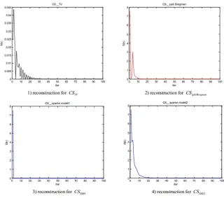
[image:3.612.130.488.245.335.2]

Experiment 1 Simulation

Figure 1. Simulation for DMU.

MN measurement matrix is extracted from sample matrix with single pixel camera experiment in Rice University, test data by yk Axk Set M 2048, N 4096, K 10, F 2. The simulation

results of algorithms are given in Fig 1. Fig 2 shows the convergences of CS_TV ,CS_splitBregman,CS_SSB1

and CS_SSB2.

[image:3.612.149.469.433.716.2]

Experiment 2 Measurement Data Reconstruction

[image:4.612.154.465.122.204.2]

Measurement data obtained by experiment Rice single pixel camera makes. The reconstructed data experiments based on CSTVand CSSSB2are given in Fig 3.

Figure 3. Synthetic data reconstruction.

0 10 20 30 40 50 60 70 80 90 100

0 0.005 0.01 0.015 0.02 0.025 0.03

CS__TV&CS__sparse model2 reconstruction for R

iter

(

k)

[image:4.612.338.499.252.385.2]

CS-TV CS-Model2

Figure 4. Convergence for CSTVand CSSSB2.

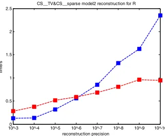
10^-30 10^-4 10^-5 10^-6 10^-7 10^-8 10^-9 10^-10 0.5

1 1.5 2 2.5

CS__TV&CS__sparse model2 reconstruction for R

reconstruction precision

tim

e/s

Figure 5. The relationship between accuracy and time.

Conclusion

Compared to other algorithm, Minimum total variation always maintains good convergence for different images and measurement data, and can obtain fine quality of images, which are susceptible to the effects of measurement noise. For split Bregman, the parameters of μ and  determine the qualities of images recovery, precision and the speed of convergence. Likewise, the control

item T T 1

A AA E

_{D （ } _） _{controls the performance of algorithm. Fig 4 shows the speeds of} convergence for CS_TVand CS_SSB2.

The relationship between concex accuracy and time is given in Fig 5.

Acknowledgement

This research was financially supported by the National Science Foundation.

References

[1] Yonina C. Eldar, Gitta Kutyniok. Compressed sensing theory and applications., Cambridge University Press, England, 2012.

[2] Foucart S., Rauhut H. A mathematical introduction to compressive sensing, Birkhäuser, Boston, 2013.

[image:4.612.105.272.252.385.2]

[4] Herzet C., Drémeau A. Bayesian Pursuit Algorithms 1474-1478, 2010.

[5] Schniter P., Potter L.C., Ziniel J. Fast Bayesian matching pursuit, Information Theory and Applications Workshop. 326-333, 2008.

[6] Candès E.J., Guo F. New multiscale transforms, minimum total variation synthesis: Applications to edge-preserving image reconstruction, Signal Processing. 82(11): 1519-1543, 2002.

[7] Mouyan Zou. Deconvolution and signal recovery, National defense Industry Press, Beijing, 2001.

[8] Gen Li, Chunan Tang, et al. High-efciency improved symmetric successive over-relaxation preconditioned conjugate gradient method for solving large-scale finite element linear equations, Applied Mathematics and Mechanics. 34(10) 1225-1236, 2013.

[9] Xu Y., Huang T.Z., Liu J., et al. Split Bregman iteration algorithm for image deblurring using fourth-order total bounded variation regularization model, Journal of Applied Mathematics. 2013(3) 417-433, 2013.

[10] Goldstein T., Osher S. The split Bregman method for L1-regularized problems, SIAM Journal on Imaging Sciences. 2(2) 323-34, 2009.

[11] Rubinstein R., Zibulevsky M., Elad M. Efficient implementation of the K-SVD algorithm using batch orthogonal matching pursuit, CS Technion. 40(8) 1-15, 2008.

[12] Indyk P. Explicit constructions for compressed sensing of sparse signals, Proceedings of the nineteenth annual ACM-SIAM symposium on Discrete algorithms, Society for Industrial and Applied Mathematics. 30-33, 2008.

[13] Yin W., Osher S., Goldfarb D., et al. Bregman iterative algorithms for l1 minimization with