Optimization over an integer efficient set
of a Multiple Objective Linear Fractional
Problem
Zerdani, Ouiza and Moulai, Mustapha
University Mouloud Mammeri, Algeria, University of USTHB,
Algeria
10 February 2011
Online at
https://mpra.ub.uni-muenchen.de/35579/
Optimization over an Integer Efficient Set
of a Multiple Objective Linear Fractional Problem
Ouiza Zerdani
University Mouloud Mammeri, Laboratory LAROMAD Faculty of Sciences, Tizi-Ouzou, Algeria
Mustapha Moulai
University of USTHB, Laboratory LAID3 Faculty of Mathematics, Algeria
mustapha [email protected]
Abstract
The problem of optimizing a real valued function over an efficient set of the Multiple Objective Linear Fractional Programming problem (MOLFP) is an important field of research and has not received as much attention as did the problem of optimizing a linear function over an efficient set of the Multiple Objective Linear Programming problem (MOLP).In this work an algorithm is developed that optimizes an arbi-trary linear function over an integer efficient set of problem (MOLFP) without explicitly having to enumerate all the efficient solutions.The proposed method is based on a simple selection technique that improves the linear objective value at each iteration.A numerical illustration is included to explain the proposed method.
Mathematics Subject Classification: 90C10; 90C26; 90C32; 90C29
Keywords: Integer programming, Optimization over the efficient set, Mul-tiple objective linear fractional programming, Global optimization
1
Introduction
However, Integer Linear Fractional Programming problem with Multiple Objective (MOILFP) has not received as much attention as did the multiple objective linear fractional programming (MOLFP).To our knowledge there are very few algorithms [1,10,23] for (MOILFP) taking into account the integrity of the variables.Affine fractional functions as widely used as performance mea-sures in some management situations, production planning and the analysis of financial enterpries.Thus the multicriteria programming problems with affine fractional criterion functions are important and have wide applications in var-ious fields as financial planning [3], transportation problem [12], manpower planning models[19].
Mathematically, (MOILFP) is described as the problem of finding all effi-cient solutions of the problem
maximize{Z1(x) =
p1
x+α1
q1x+β1}
maximize{Z2(x) =
p2
x+α2
q2x+β2} (P)
.. .
maximize{Zr(x) =
prx+αr
qrx+βr}
subject to x∈S,
where αi,βi are scalars; pi, qi∈Rn for each i∈ {1,2, ..., r};S=D∩Zn;r≥2;
D ={x∈Rn/Ax≤b, x≥0}; b∈Rm; A∈Rm×n; Z is the set of integers.
It is assumed that S is not empty and D is a bounded convex polyhedron in
Rn and qix+βi>0 over D for all i∈ {1,2, ..., r}.
The set of all integer efficient solutions of (P) is denoted by E(P).
As in multiple objective linear programming see [24,25], the solution to the problem (P) is to find all solutions that are efficient in the sense of the following definition.
Definition 1.1 A point x0
∈ S is said to be efficient of (P) if and only if there does not exist another point x1 ∈
S such that Zi(x1) ≥ Zi(x0) for all
i∈ {1,2, ..., r} and Zi(x1)> Zi(x0) for at least one i∈ {1,2, ..., r}.
Otherwise, x0
is called a dominated solution and the vector (Z1(x0), Z2(x0), ..., Zr(x0)) is said a dominated r−tuple.
structure of E(P).Since in many cases the criteria are in conflict,the decision maker try to optimize a linear function representing his preferences over the efficient set E(P).The problem of finding a most preferred (with respect toϕ) efficient point can be stated as a mathematical programming problem
⎧
⎪ ⎨
⎪ ⎩
maximize ϕ =d.x
s.t. x∈E(P) (PE)
where dx is a linear function (d∈Rn).
Mathematically, the problem (PE) can be classified as a global
optimiza-tion problem.The main difficulty of this problem arises from the fact that its feasible domain, in general, is nonconvex and not given explicitly.
In the continuous case, the problem of optimizing a real valued function over an efficient set of the Multiple Objective Linear Programming problem (MOLP) have attracted much attention because of their important applica-tions in decision making. This problem was first considered by Philip [22] in which an algorithm based on moving to adjacent efficient vertices is outlined.In Isermann and Steuer [16] the main idea of the algorithm is based on the use of a cutting plane procedure.Benson [4,5] has given two relaxation algorithms for solving this problem.The survey of Yamamoto [28] proposes a classification of the existing algorithms for optimization over the efficient set.Thi, Pham and Thoai [26] propose a branch and bound procedure based on some properties in Lagrange duality.Yamada, Tanino, Inuiguchi [27] propose a method for approx-imate minimization of a convex function over the weakly efficient set.Benson [6] suggested a more simple linear programming procedure for detecting and solving the problem in four special cases and many others references.
Although the discrete case has by no means seen a similar development.Linear functions optimization on an integer efficient set of (MOLP) is considered only by Nguyen [21] which gives an upper bound for the optimal objective value of the function ϕ.Abbas and Chaabane [2] where different types of cuts are imposed in such a way that the improvement of the objective value is guaran-teed at each iteration.Chaabane and Pirlot [9]; Jesus M. Jorge [17] propose an algorithm which defines a sequence of progressively more constrained single-objective integer problems that successively eliminates undesirable points from further consideration.
Problem (PE) of optimizing a linear function over a set of a vector affine
The central problem of interest in this paper is the problem of optimizing a linear function ϕ over the efficient set E(P) of problem (MOILFP).This problem is formulated as
⎧
⎪ ⎨
⎪ ⎩
Maximize w=d.x
s.t. x∈E(P) (PE)
The problem (Pi(S)), i ∈ {1,2, ..., r} is the following integer linear
frac-tional programming problem
⎧
⎪ ⎪ ⎨
⎪ ⎪ ⎩
maximize Zi(x) = p
ix+αi
qix+βi
s.t . x∈S =D∩Zn (P
i(S))
The outline of the paper is as follows:In this section we have presented the motivation for developing the approach.Section 2 compiles the notation and definitions used throughout the manuscript.In section 3, some preliminary results are given to justify the methodology.The detailed presentation of the algorithm is given in section 4.In section 5, a numerical illustration is included to explain the proposed method.
2
Notation and definitions
Along the present paper, the following notations will be used.
- D1 ={x∈ Rn1 : A1x ≤b1;A1 ∈Rm1×n1;b1 ∈ Rm1;x≥ 0}. D1 is a current
truncated region of D obtained by successive Gomory cuts introduced when optimizing problem (P1(S)). Note thatS1 =S =D1∩Zn, because
Gomory cuts do not eliminate integer solutions from D.
- (Z1 1, Z
1 2, ..., Z
1
r) is the first non-dominated r−tuple corresponding to the
op-timal integer solution x1
1 obtained inD1, whereZi1 = p
ix+αi
qix+βi
for i= 1,2, ..., r.
Fork ≥2 ,we have:
- Dk = {x ∈ Rnk : Akx ≤ bk;Ak ∈ Rmk×nk;bk ∈ Rmk;x ≥ 0}. Dk is the
current truncated region obtained after having applied the cut
j∈Nk−1\{jk−1}xj ≥1 where jk−1 ∈Γk−1 (see below) and successive
Go-mory cuts eventually.
- x1
k = (x
1
k,j) the kth optimal integer solution of problem P1(S) obtained on
Dk at stepk. ( Note that in place of (P1(S)), one can similarly consider
- B1
k is a basis associated with solution x
1
k.
- a1
k,j ∈Rmk×
1
is the activity vector ofx1
k,j with respect toDk.
- y1
k,j = (y
1
k,ij) = (B
1
k)−
1 ×a1
k,j where y
1
k,j ∈Rmk×1
- Ik={i/a1k,i∈B
1
k} (indices of basic variables)
- Nk ={j/a1k,j ∈/B
1
k} (indices of non-basic variables)
- p1
j = the jth component of vector p
1
- q1
j = the jth component of vector q
1
- p1
k,j =
i∈Ikp
1
i ·y
1
k,ij
- q1
k,j =
i∈Ikq
1
i ·y
1
k,ij
- Z1(x1k) =
Z1
k,1 Z1
k,2 = p1x1
k+α1
q1x1
k+β1
- γ1
k,j =Z
1
k,2(p 1
j−p
1
k,j)−Z
1
k,1(q 1
j−q
1
k,j) , the updated value of thejthcomponent
of the reduce gradient vector γ1
k.
- xu
k = (xuk,j) are the (tk −1) alternate integer solutions to x1k, if they exist,
where tk is an integer number and u∈ {2, ..., tk}.
- Γk = {j ∈ Nk / γ1k,j ≤ 0 and ϕkj −dkj ≤ 0}, where ϕkj =dB1
k.y
1
k,j with
dB1
k the vector of cost-coefficients of basic variables associated with B
1
k
in vector dk.
Theorem 2.1 [20] The point x1
k of S is an optimal solution of problem
(P1(S)) if and only if the reduce gradient vector γ 1
k is such that γ
1
k,j ≤0for all
j ∈Nk.
Remark 2.2 Recall that a sufficient condition for the uniqueness of the optimal solutionx1
k of (P1(S))is that the set Jk={j ∈Nk/γ1k,j = 0} is empty.
In this case, there does not exist any other integer feasible solution x inS
such that Z1(x) = Z1(x1k). We refer to x as an alternate optimal solution to
x1
k.
We recall a well known result[22].
Corollary 2.3 A pointx0
3
Theoretical results
Since the problem MOILFP is to determine the set of integer efficient solutions, we scan all integer points of the feasible region S by a cutting plane technique which is described in the present section.
Definition 3.1 Assume that jk ∈ Nk. An edge Ejk incident to a solution
x1
k is defined as the set
Ejk =
⎧
⎪ ⎪ ⎪ ⎪ ⎪ ⎪ ⎨
⎪ ⎪ ⎪ ⎪ ⎪ ⎪ ⎩
x= (xi)∈Dk :
⎧
⎪ ⎪ ⎪ ⎨
⎪ ⎪ ⎪ ⎩
xi =x1k,i−θjk.y
1
k,ijk for i∈Ik
xjk =θjk
xv = 0 for all v ∈Nk\{jk}
(1)
where 0< θjk ≤mini∈Ik{
x1
k,i
y1
k,ijk/y
1
k,ijk >0}, θjk is a positive integer and θjk.y
1
k,ijk are integers for all i∈Ik if such integer values exist.
Remark 3.2 Note that equation (1) enables us to compute the integer fea-sible alternate solutions when the optimal solution obtained by solving (P1(S))
is not unique (Jk=∅).
The following theorem addresses the case in which the optimal solution of (P1(S)) is not unique.
Theorem 3.3 [1]All integer feasible solutionsxu
k, u∈ {2, ..., tk}of problem
(P1(S)) alternate to x1k on an edge Ejk of region D (or truncated region Dk) emanating from it, in the direction of a vector a1
k,jk, jk ∈Jk, exist in the open half space.
j∈Nk\{jk}
xj <1 (2)
The following theorem suggests a cut that can be viewed as a generalization of Dantzig’s cut.
Theorem 3.4 [1] An integer feasible solution of problem (P1(S)) that is
distinct from x1
k and not on an edge Ejk, jk ∈ Jk of the truncated region
Dk (or D)through an integer feasible point xk1 of problem (P1(S))exists in the
closed half space
j∈Nk\{jk}
1- We calculate the value ϕ′
k of the linear function ϕ at any solution
xu
k = (xu1, xu2, ..., xun) lying on the edgeEjk.
ϕ′k =
n j=1 dk j.x u j =
i∈Ik
dk
i(xk,i−θjk.yk,ijk) +d
k jk.θjk
ϕ′k = (d k jk−
i∈Ik
dki.yk,ijk).θjk +
i∈Ik
dki.xk,i
where θjk is an integer verifying 0< θjk ≤θ
0
jk and θ
0
jk is the integer part
of mini∈Ik{
xk,i
yk,ijk/yk,ijk >0}.
We put :
υk= (dkjk−
i∈Ik
dk
i.yk,ijk) (4)
Then along an edge Ejk, jk ∈Γk, we have υk ≥0. Therefore, the values
of ϕ′
k are increasing and ϕ′k reaches its maximum forθjk =θ
0
jk.
Definition 3.5 Let f : S ⊂ Rn−→R and x∈ S. Then
L≥f(x) ={x∈S :f(x)≥f(x)} is called the level set of x for f.
L=f(x) ={x∈S :f(x) =f(x)} is called the level curve of x for f.
2- The following theorem is used in various steps of our algorithm to test the efficiency of a given integer feasible solution of Multiobjective Integer Linear Fractional Programming problem (P).
Theorem 3.6 [14]Characterization of Pareto optimal solutions
x∈S is Pareto optimal of (P) if and only if i
=r
i=1
L≥Zi(x) = i=r
i=1
L=Zi(x).
Proof: x is Pareto optimal of (P)
⇐⇒T here does not exist x∈S such that [Zi(x)≥Zi(x) ∀ i= 1...r
and Zj(x)> Zj(x) f or some j]
⇐⇒T here does not exist x∈S such that [x∈i=r
i=1L≥Zi(x) and ∃ j :x∈L>Zj(x)]
⇐⇒i=r
i=1
L≥Zi(x) = i=r
i=1
L=Zi(x)
3- Before starting the description of the algorithm we introduce the following inequality (dx ≥ ϕopt) which eliminate only solutions that are strictly
4
Development of the algorithm
The algorithm that we propose here is proved to provide an optimal solution of (PE) without having to compute the set of all efficient solutions of the
underlying problem (P).
Step 0: Initialization let ϕopt =−∞
Solve the relaxed problem (PR) : max{dx / x∈S}
- If (PR) is unfeasible⇒ STOP, (PE) is unfeasible.
- Otherwise, let x0
be an optimal solution of (PR).
Step 1: This solution is tested for efficiency by applying the Theorem 3.6
- If x0
∈E(P)⇒ STOP, x0
is an optimal solution of (PE).
- Otherwise, go to step 2.
Step 2: Solve the problem (P1(S)) [one may similarly consider any of the
problems (Pi(S)) i= 2,3, ..., r instead of (P1(S))].
2.1 If J1 = {j ∈ N1/γ11,j = 0} = ∅ then the optimal solution found x
1 1 is
unique and it is efficient (corollary 2.3). Set (xopt = x11,ϕopt = dx11) and
go to step 3.
2.2 If J1 =∅ then x11 may not be unique, test the efficiency of x 1 1.
- If it is not efficient go to step 3.
- Otherwise, set (xopt =x11, ϕopt = dx11) and go to step 3.
Step 3: Let k= 1 and perform the following sub-steps:
3.1 Construct the set Γk={j ∈Nk/γkk,j ≤0 and ϕkj −dkj ≤0}.
− If Γk =∅, then go to step 3.3 and apply the Dantzig cutj∈Nkxj ≥1.
− Otherwise, letγ = Γk. go to (a).
a - If γ =∅, then let jk∈Γk and go to 3.3.
- Else, select jk∈γ and calculate θ0jk the integer part of
mini∈Ik{
x1
k,i
y1
k,ijk/y
1
k,ijk >0}
- If θ0
jk = 0 then there is no integer feasible solution on the
edge Ejk, put γ =γ\{jk} and go to (a).
- Else, if θ0
b - If x1
k is efficient and dx
1
k ≥ ϕopt, then calculate the value
of the parameter υk defined in equation (4).
- If υk = 0, then go to (c).
- If υk = 0, put γ =γ\{jk} and go to (a).
- If x1
k is not efficient or dx
1
k< ϕopt, then go to (c).
c- Explore the edge Ejk, searching for a feasible integer
so-lutions of (P1(S)) corresponding to θjk (θjk is an integer
verifying 0< θjk ≤θ
0
jk) and test for efficiency starting from
θjk =θ
0
jk until θjk = 1.
Once a first integer efficient solution is found, say xu k such
that dxu
k > ϕopt, set (xopt = xku, ϕopt = dxuk), and go to
sub-step 3.2.
If there is no integer efficient solution on this edge, then put γ =γ\{jk}and go to (a).
3.2 Letk =k+ 1. Define the new truncated regionDk as the subset of Dk−1
obtained by applying the cut (dx ≥ dxu
k−1) and using the dual simplex
method and gomory cuts, if necessary, to find a new optimal solution
x1
k.Set (xopt =x1k, ϕopt =dx1k) and go to (3.1).
3.3 Let k = k+ 1. The new truncated region Dk is obtained as a subset of
Dk−1 by applying the specified cut (Dantzig cut j∈Nkxj ≥ 1 or cut
j∈Nk\{jk}xj ≥1) and using the dual simplex method and Gomory cuts,
if necessary, to find a new optimal solution x1
k.
- If the solutionx1
k is efficient anddx
1
k> ϕopt, set (xopt =xk1,ϕopt =dx1k)
and go to (3.1)
- Else, go to (3.1).
Terminal step: The process terminates when infeasibility of pivot operations appears indicating that the current region contains no integer feasible pointx1
k
such that dx1
k > ϕopt. The optimal solution of problem (PE) is then xopt and
its value on criterion ϕ is ϕopt.
Proposition 4.1 Under the hypothesis that Sis not empty and Dbounded, the algorithm ends up with an efficient solution of problem (P).
Proof: Since D is bounded, S is non-empty and finite. Each cut of Dantzig
j∈Nkxj ≥ 1 or a cut of type
j∈Nk\{Jk}xj ≥ 1 reduces strictly the domain.
Theorem 4.2 If S is non-empty and D is bounded, then
1. The algorithm terminates in a finite number of iterations.
2. The solution xopt is an optimal solution of problem (PE).
Proof: Proposition (4.1) guarantees that we can obtain an initial efficient solution of (P), at iteration p, p≥1. We see also from the description of the algorithm that, during iteration k, either a cut of Dantzig
j∈Nkxj ≥ 1 or a
cut of type
j∈Nk\{Jk}xj ≥1 is applied which strictly reduces the domain or a
new efficient solution is found that improves ϕopt. Obviously, since the domain
S is finite, it may not be strictly reduced an infinite number of times. For the same reason, only a finite number of improvements ofϕ =dxmay be observed when x moves in the finite set S. This proves that the algorithm stops after a finite number of iterations.
ProvidedSis non-empty andDis bounded, the algorithm stops at iteration
k > pif and only if the problem (P1(Sk)) is unfeasible, this is seen from the fact
that, the dual simplex algorithm, at some stage, possibly after the adjunction of Gomory cuts, can not perform any pivot operation. The current value of
ϕopt at that iteration is optimal and xopt is an optimal solution of problem
(PE).
5
Numerical illustration
To illustrate the use of this algorithm, we consider the following integer linear fractional program with three objectives [18].
Maximize Z1(x) =
−x1+ 4
x2+ 1
;Z2(x) =
x1 −4 −x2 + 3
;Z3(x) =−x1+x2
(P)
subject to x∈S where
S= x∈R2
:−x1 + 4x2 ≤0;x1−
1
2x2 ≤4;x1, x2 ≥0 and integers
Let the main problem be
⎧
⎪ ⎨
⎪ ⎩
max ϕ= 2x1−3x2 (PE)
Step 0: Initialization Letϕopt=−∞
We solve the relaxed problem (PR)
⎧
⎪ ⎨
⎪ ⎩
max(2x1 −3x2)
x∈S
The optimal solution is x0
= (4,0)′ and ϕ0
= 8.
Step 1: This solutionx0
is tested for efficiency ( theorem 3.6) and we obtain:
3
i=1
L≥fi(4,0) = {(4,0)′; (4,1)′} =
3
i=1
L=fi(4,0) ={(4,0)′}
Thus x0
is not efficient go to step 2.
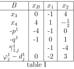
Step 2: We solve the problem (P1(S))
⎧
⎪ ⎨
⎪ ⎩
max(−x1+4 x2+1 )
x∈S
The results of solving problem (P1(S)) using the procedure developed in [7] or
[15] are summarized in table I.
B xB x1 x2
x3 0 -1 4
x4 4 1 −
1 2
-p1
-4 -1 0 -q1
-1 0 1
γ1
1,j -1 -4
ϕ1
j−d
1
[image:12.612.236.363.353.471.2]j 0 -2 3
table I
The optimal solutionx1
1 = (0,0)′ is unique, thus it is efficient. Let it be a first
efficient solution that corresponds to ϕ1
= 0. We have dx1
1 = 0 > −∞ then
ϕopt = 0 andxopt = (0,0)′.
Step 3: 3.1 k = 1
I1 = {3,4}; N1 = {1,2}, Γ1 ={j ∈ N1/γ11,j ≤ 0 and ϕ
1
j −d
1
j ≤ 0} =
{1} =∅. We put γ = Γ1 ={1}.
Let j1 = 1 ∈γ. Since x 1
1 is efficient and dx 1
1 = 0 > ϕopt =−∞ then we
calculate the value of υ1.
υ1 =d11−d 1
3.y1,31−d13.y1,41= 2−0.(−1)−0(1) = 2>0, we start exploring
the edge E1; we calculate θ 0
1 = min{ 4
1} = 4 ; for θ1 = 4 , x 2
1(4) = (4,0)′
which is not efficient.
corresponding solution an the edge E1 is x31(3) = (3,0)′.
The solution x3
1(3) is being tested for efficiency and we obtain:
3
i=1
L≥fi(3,0) =
3
i=1
L=fi(3,0) ={(3,0)′}
Thus x3
1(3) is efficient. We calculate ϕ 1 1 =d.x
3
1(3) = 6.
As ϕ1
1 > ϕopt = 0, then ϕopt= 6 and xopt = (3,0)′.
3.2 k =k+ 1 = 2
We cut by 2x1−3x2 ≥6
After adjusting the table I for the reduced feasible region and applying the dual simplex method.The optimal feasible solution is x1
2 = (3,0)′
which is efficient. It corresponds to ϕ2
= 6; ϕopt = 6 and xopt = (3,0)′
(see table II)
B xB x2 x5
x3 3
5 2 −
1 2
x4 1 1 12
x1 3 −
3 2 −
1 2
-p2
-1 −3 2 −
1 2
-q2
-1 1 0
γ1
2,j −
5 2 −
1 2
ϕ2
j −d
2
j 6 0 -1
table II
I2 ={1,3,4}, N2 ={2,5}, Γ2 ={2,5} =∅
Let γ = Γ2. Let j2 = 2. Since x12 is efficient and dx 1
2 = ϕopt = 6, then
we calculate the value of υ2; υ2 =−3−(2(− 3
2) + 0 + 0) = 0.We do not
explore the edge E2.
Let γ =γ\{2} and consider the second index j2 = 5 ∈γ ,θ50 = min{ 1
1 2
}
= 2 .Since x1
2 is efficient anddx2 =ϕopt = 6, then we calculate the value
of υ2; υ2 = 0−(2×(− 1
2)) = 1>0 we explore the EdgeEj2 =E5. The corresponding solution on the edgeE5 isx22(2) = (4,0) which is not
efficient and x3
2(1) = ( 7
2,0) which is not integer.
We have γ =γ\{5}=∅.
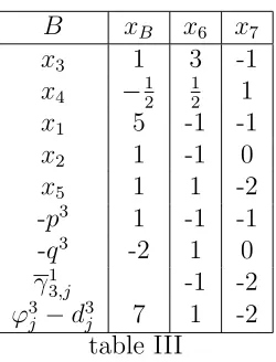
3.3 Let k=k+ 1 = 3
and we cut the current feasible region by
B xB x6 x7
x3 1 3 -1
x4 −12 12 1
x1 5 -1 -1
x2 1 -1 0
x5 1 1 -2
-p3
1 -1 -1 -q3
-2 1 0
γ1
3,j -1 -2
ϕ3
j −d
3
[image:14.612.252.377.71.235.2]j 7 1 -2
table III
The dual is not feasible then the algorithm terminates.
The optimal solution of problem (PE) is thenxopt = (3,0)′ and ϕopt = 6.
This example was first presented in [18] to find the set of integer efficient solutions : E(P) = {(4,1)′; (3,0)′; (2,0)′; (1,0)′; (0,0)′}.
However, our algorithm optimizes the linear function ϕ = 2x1 − 3x2
without having to determine all these solutions but only {(0,0)′,(3,0)′}.
6
Conclusion
In this work we have presented a new algorithm for optimizing a linear func-tion over an efficient set of the Multiple Objective Integer Linear Fracfunc-tional Programming problem (MOILFP).
The proposed algorithm solves problem (PE) by using classical linear
program-ming procedures without having to enumerate all the efficient solutions. The algorithm may generate several dominated solutions but it provides a shorter way to the optimal one.
References
[1] M. Abbas and M. Moulai, Integer linear fractional programming with multiple objective,Journal of the Italian Operations Research Society, 32 (2002), N◦103−104,15−38.
[3] D.J. Ashton and D.R. Atkins, Multicriteria programming for financial planning, Journal of the Operational Research Society, 30 (1989), N◦3, 259-270.
[4] H.P. Benson, An All-Linear Programming Relaxation Algorithm for Op-timizing over the Efficient Set,Journal of Global Optimization, 1 (1991), 83-104.
[5] H.P. Benson, A finite Nonadjacent Extreme Point Search Algorithm over the Efficient Set, Journal of Optimization Theory and Applications, 73 (1992), N◦1, 47-64.
[6] H.P. Benson and S. Sayin, Optimizing over the Efficient Set: Four Special Cases,Journal of Optimization Theory and Applications,80(1994), N◦1, 3-17.
[7] A. Cambini and L. Martein, A modified version of Martos’algorithm for the linear fractional problem, Mathematics of Operations Research, 53 (1986), 33-44.
[8] A. Cambini, L. Martein and I.M. Stancu-Minasian, A survey of bicriteria fractional problems,Advanced Modeling and Optimization, 1(1999), N◦1, 9-46.
[9] D. Chaabane and M. Pirlot, A method for optimizing over the integer efficient set,Journal of industrial and management optimization,6(2010), N◦4, 811-823.
[10] M.E.A. Chergui and M. Moulai, An exact method for a discrete multi-objective linear fractional optimization, Journal of Applied Mathematics and Decision sciences, 2008 (2008), Article ID 760191,12 pages.
[11] J.P. Costa, Computing non-dominated solutions in MOLFP, European Journal of Operational Research, 181 (2007), N◦3, 1464-1475.
[12] N. Datta and D. Bhatia, Algorithm to determine an initial efficient basic solution for a linear fractional multiple objective transportation problem,
Cahiers Centre Etudes Rech.Oper., 26 (1984), N◦1−2, 127-136.
[13] J.G. Ecker and J.H. Song, Optimizing a Linear Function over an Efficient Set, Journal of Optimization Theory and Applications, 83 (1994), N◦3, 541-563.
[15] D. Granot and F. Granot, On integer and mixed integer fractional pro-gramming problems, Annals of Discrete Mathematics, 1 (1977), 221-231.
[16] H. Isermann and R.E. Steuer, Computational Experience Concerning Pay-off Tables and Minimum Criterion Values over the Efficient Set,European Journal of Operational Research, 33 (1987), 91-97.
[17] J.M. Jorge, An algorithm for optimizing a linear function over an integer efficient set, European Journal of Operational Research, 195 (2009), 98-103.
[18] J.S.H. Kornbluth and R.E. Steuer, Multiple objective linear fractional programming, Management Science, 27 (1981), N◦9, 1024-1039.
[19] J.S.H. Kornbluth, Ratio goals in manpower planning models, INFOR-canad.J.Oper.Res.Inform.Process., 21 (1983), N◦2, 151-154.
[20] B. Martos, Hyperbolic Programming,Naval Res.Logist.Quart.,11(1964), 135-155.
[21] N.C. Nguyen, An Algorithm for Optimizing a Linear Function over the In-teger Efficient Set, Konrad-Zuse-zentrum fur Informationstechnik Berlin,
(1992).
[22] J. Philip, Algorithms for the vector maximization problem, Mathematical programming,2 (1972), 207-229.
[23] O.M. Saad and J.B. Hughes, Bicriterion integer linear fractional programs with parameters in the objective functions, Journal of Information and optimization Sciences,19 (1998), N◦1, 97-108.
[24] R.E. Steuer, Multiple criteria optimization: Theory, computation and ap-plication,Wiley Series in probability and Mathematical Statistics: Applied Probability and Statistics, John Wiley and Sons, Inc.XXII, New York, 1986.
[25] J. Teghem and P. Kunsch, A survey of techniques to determine the effi-cient solutions to multi-objective integer linear programming,Asia Pacific Journal of Operations Research, 3 (1986), 95-108.
[26] H.A.L. Thi, D.T. Pham and N.V. Thoai, Combination between Global and Local Methods for Solving an Optimization Problem over the Efficient Set,
[27] S. Yamada, T. Tanino and M. Inuiguchi, An Inner approximation method Incorporating a Branch and Bound procedure for Optimization over the Weakly Efficient Set, European Journal of Operational Research, 133 (2001), N◦2, 267-286.
[28] Y. Yamamoto, Optimization over the Efficient Set: overview, Journal of Global Optimization, 22 (2002), N◦1−4, 285-317.