Diffusion Process of High Concentration Spikes in a Quasi Homogeneous Turbulent Flow

ISSN Online: 2165-3860 ISSN Print: 2165-3852

Diffusion Process of High Concentration Spikes in

a Quasi-Homogeneous Turbulent Flow

Masaya Endo, Qianqian Shao, Takahiro Tsukahara, Yasuo Kawaguchi

Department of Mechanical Engineering, Tokyo University of Science, Chiba, Japan

Abstract

When a mass spreads in a turbulent flow, areas with obviously high concentration of the mass compared with surrounding areas are formed by organized structures of turbulence. In this study, we extract the high concentration areas and investigate their diffusion process. For this purpose, a combination of Planar Laser Induced Fluorescence (PLIF) and Particle Image Velocimetry (PIV) techniques was employed to obtain simultaneously the two fields of the concentration of injected dye and of the velocity in a water turbulent channel flow. With focusing on a quasi-homogeneous turbulence in the channel central region, a series of PLIF and PIV images were ac-quired at several different downstream positions. We applied a conditional sampling technique to the PLIF images to extract the high concentration areas, or spikes, and calculated the conditional-averaged statistics of the extracted areas such as length scale, mean concentration, and turbulent diffusion coefficient. We found that the av-eraged length scale was constant with downstream distance from the diffusion source and was smaller than integral scale of the turbulent eddies. The spanwise distribution of the mean concentration was basically Gaussian, and the spanwise width of the spikes increased linearly with downstream distance from the diffusion source. Moreover, the turbulent diffusion coefficient was found to increase in proportion to the spanwise distance from the source. These results reveal aspects different from those of regular mass diffusion and let us conclude that the diffusion process of the spikes differs from that of regular mass diffusion.

Keywords

Turbulent Transport, High Concentration Spikes, Quasi-Homogeneous Turbulent Flow, Conditional Sampling Technique, PIV and PLIF Measurements, Passive Scalar Diffusion

1. Introduction

Understanding the turbulent transport of passive scalar is very important in environ-How to cite this paper: Endo, M., Shao,

Q.Q., Tsukahara, T. and Kawaguchi, Y. (2016) Diffusion Process of High Concen-tration Spikes in a Quasi-Homogeneous Tur- bulent Flow. Open Journal of Fluid Dynam-ics, 6, 371-390.

http://dx.doi.org/10.4236/ojfd.2016.64028

Received: October 14, 2016 Accepted: December 23, 2016 Published: December 26, 2016

Copyright © 2016 by authors and Scientific Research Publishing Inc. This work is licensed under the Creative Commons Attribution International License (CC BY 4.0).

http://creativecommons.org/licenses/by/4.0/

mental flows where pollutants affect the safety and quality of our life. For instance, dif-fusion accidents have affected a large number of victims around the world, as in the Chernobyl Nuclear Power Plant disaster in 1986 and the Fukushima Daiichi Nuclear Power Plant in 2011. In such cases, a quick and accurate method of predicting pollutant diffusion is needed in order to prevent damages. As an example of prediction method for substance’s diffusion, the SPEEDI (System for Prediction of Environmental Emer-gency Dose Information) was applied when radioactive material was emitted from the Fukushima Daiichi Nuclear Power Plant [1] [2] [3]. For realization of the diffusion prediction, the diffusion theory in turbulent flows has been studied for many years. There are pioneering studies on the diffusion theory such as Taylor’s diffusion theory [4] and Richardson’s diffusion theory [5]. These theories reference the spreading width of a diffusing material released into homogeneous turbulence, revealing that the rela-tionship between the increasing rate of the spreading width and the diffusion time de-pends on whether the diffusion time is smaller or larger than the time scale of eddies in the flow. The relationship has been investigated further with time-average scalar statis-tics including mean concentration, concentration fluctuation intensity and the turbu-lent diffusion coefficient by experimental and numerical methods [6][7][8][9]. Owing to the progress of research on the diffusion theory, the diffusion prediction has become more accurate and speedy.

spikes is an important challenge in reducing the damage from pollutant diffusion by means of a quick localization of the emission source.

In this paper, we worked out the basic diffusion theory of the high concentration spikes in a turbulent flow based on Taylor’s diffusion theory. Taylor’s diffusion theory deals with a suspended single particle emitted from a point source and assumes the homogeneous turbulence without any external body force such as buoyancy. With the aim of calculating the scalar statistics of high concentration spikes, which relate to the diffusion theory, we experimentally demonstrated the concentration and velocity fields of passive scalar (dye) diffusing from a fixed emission point in a quasi-homogeneous turbulent flow with simultaneous PIV (Particle Image Velocimetry) and PLIF (Planar Laser Induced Fluorescence) measurement. As a simple test case, we employed a water channel flow between two parallel walls. The high concentration spike we focus on in this study occurs intermittently in the turbulent flow, and its unconditional statistical quantities such as mean concentration and concentration fluctuation cannot be calcu-lated by the normal ensemble-average operation. In order to extract the high concen-tration spikes, the conditional sampling technique [16] was applied to a spatial dye- diffusion image obtained by PLIF measurement. From the experimental results of the scalar statistics of the extracted spikes, which include spanwise diffusion width, average length scale, mean concentration, and turbulent diffusion coefficient, the diffusion theory of the spikes as well as its difference with that of the concentration plume were discussed.

2. Experimental Procedure

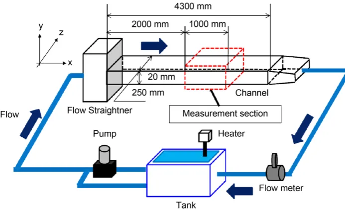
Figure 1 shows a schematic diagram of our main experimental apparatus, which was a closed-circuit water channel. The water flow under constant temperature was driven by an inverter controlled centrifugal pump with the constant volume. A rectifier was in-stalled at the entrance to ensure a steady flow by damping the large vortices. The chan-nel part including the measurement section was made of transparent acrylic resin for precise visualization and had a height of 20 mm (2δ), and a width of 250 mm (aspect ratio 12.5). A fully developed two-dimensional turbulent channel flow was established in the measurement section, which was located 2000 - 3000 mm downstream from the channel inlet. The flow rate Q was measured by a flow-meter to monitor the constant Reynolds number. The bulk Reynolds number was fixed at Reb=2Ubδ ν =20000, where Ub

(

(

)

)

In this study, we focus on the statistically modeled quasi-homogeneous turbulence to investigate the fundamental characteristics of the high concentration spikes. Accor-dingly, the uniformities of the time-average velocity and turbulent intensity in the tur-bulent flow are important. Figure 2 shows the spanwise distributions of time-average streamwise velocity Uc and turbulent intensity urms′ at the channel center obtained by

Figure 1. Experimental apparatus.

Figure 2. Spanwise distributions of time-average streamwise ve-locity and turbulent intensity at channel center obtained by PIV measurement.

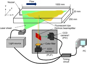
acceptable. This means that the flow field we focus on in this study is quasi-homogeneous turbulence in the two-dimensional plane of the streamwise and spanwise directions. In order to measure the spatial velocity field and concentration field at the same time and at the same position, we employed simultaneous PIV and PLIF measurement.

Figure 3. Measurement section for simultaneous PIV and PLIF measurement.

[20]. For a reference, note also that the streamwise integral length scale obtained by in-tegration of the streamwise two-point correlation coefficient was about 0.7δ.

3. Analysis Method

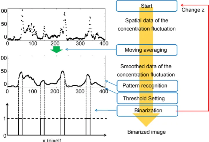
To calculate the scalar statistics of the high concentration spikes it is necessary to indi-cate the position and area of the spikes in the PLIF image describing the diffusing dye. In this study, a conditional sampling technique was used, which comprised the moving av-eraging, pattern recognition and binarizing by setting a threshold, as shown in Figure 4. Firstly, spatial data on concentration fluctuation C'(x, z) were obtained for different x at a fixed z from the raw PLIF images. Then C'(x, z) was smoothed by the moving averag-ing method [21].

We assumed that the spikes were formed by the large-scale structure of turbulent ed-dies, and employed the smoothing window length NL (=LE/Δx) consisting of streamwise integral length scale LE and spatial resolution Δx of the photograph image. After that, by applying pattern recognition to the smoothed data, the corresponding waveform pattern was extracted. When the maximum value of concentration fluctuation in the waveform pattern recognized by the pattern recognition was higher than the threshold of concen-tration, the waveform pattern was extracted. In this technique, the threshold was the root mean square of C'(x, z). Thereafter, the concentration on the extracted waveform pattern was binarized as either zero or one: the concentration between the position of the largest gradient and the smallest gradient in the waveform pattern was binarized as one, while the other part was binarized as zero. When the above analysis was performed for all z on each PLIF image, the time series of the two-dimensional binarized images was obtained and the spikes were extracted. This spike extraction method is based on

both the concentration values and gradients, proposed in [16] by the authors. There are two notable points: that the conditional sampling technique doesn’t have any influence on the original image of the diffusing dye and that the versatility of the technique has a limit that the technique can be applied only when intended flow is homogeneous and steady.

4. Results and Discussion

4.1. Extraction of the High Concentration Spikes

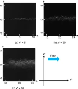
The concentration of fluorescent dye was measured by the PLIF technique around four streamwise locations: x* = 5, 20, 40, and 60. Here, the superscript of * indicates norma-lization by the channel half width, i.e., x* = x/δ. For different streamwise locations, areas of the same size were selected based on the recorded PLIF images, and the further spike statistical analysis was done focused on the selected areas.

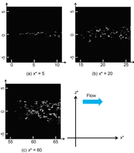
Figure 5 takes the original PLIF images for three locations for example. In Figure 5, higher brightness means higher fluorescent intensity, which is proportional to the local dye concentration. Figure 5 shows dye plumes with low and high concentration areas. Figure 6 shows the corresponding binarized images obtained by the conditional sam-pling technique mentioned above, and the length-scale mark is also shown in the figures. From Figure 5, it is found that the spanwise diffusion width of the plume spreads for downstream distance x*, which means that the diffusion of the plume progresses with

Figure 6. Binarized concentration images visualizing high concentration spikes obtained by the conditional sampling.

the diffusion time T≡ x/Uc. Here, the diffusion time of the plume is estimated using the downstream distance from the diffusion source and time-average streamwise veloc-ity under Taylor’s frozen turbulence hypothesis. In the diffusing plume, the tion fluctuates in space and there are areas having a high concentration and concentra-tion gradient compared with the surroundings. Moreover, a meandering moconcentra-tion of the diffusing plume is not identified definitely in Figure 5, which was observed under the turbulent flow background at high Reynolds numbers [22]. The occurrence of the meandering motion depends on the relationship between the Lagrangian time scale of the turbulent field and the diffusion time of the plume, and can be observed when the diffusion time is shorter than the Lagrangian time scale. In this experiment, the La-grangian time scale TL ≈ 0.036 s can be estimated by Equation (1), which was given by Hanna [23].

rms

0.25 E ,

L

L T

u

=

′ (1)

( ) (

)

( )

(

)

0 d ,

E

u x u x r

L r

u x

∞ ′ ′ +

=

′

∫

instan-taneous velocity u and the time-average streamwise velocity Uc. The Lagrangian time scale consists of the Eulerian length scale LE corresponding to the streamwise integral length scale and the streamwise turbulent intensity urms′ . The Lagragian time scale is

smaller than the shortest diffusion time T = 0.05 s among the measurement positions. Based on Taylor’s diffusion theory, in this experiment, a large part of the diffusion of the plume in the photographed areas corresponded to long-time diffusion.

The white areas in Figure 6 stand for the high concentration spikes, while the black areas indicate zero or low concentration areas. Therefore, Figure 6 shows the existence of the high concentration spikes in the diffusing plume. Note here that Figure 6 of the binarized images are obtained from Figure 5 of the original raw PLIF images by apply-ing the above-mentioned samplapply-ing technique. Comparapply-ing the correspondapply-ing original and binarized images, it can be seen that high concentration spikes are distinguished with clear outlines by extraction. Moreover, the high concentration spikes are scattered randomly in Figure 6. From Figure 5 and Figure 6, it can be seen that a large number of high concentration spikes exist even at the edge of the plume where the concentra-tion is very low.

The reason is that such a low-concentration edge area has a large concentration gra-dient, so the spikes can be recognized. Actually, through extraction by the conditional sampling technique, the low-concentration edge area of the plume is also taken se-riously, which is more reasonable than analyzing only based on the plume concentra-tion. As x* increases, the white areas appear clearer and their number increases in the image. Considering that the high concentration spikes are formed by the organized structure of turbulence and extracted by judging the plume concentration by concen-tration values as well as concenconcen-tration gradients, it can be suspected that the behavior of the spikes follows a totally different diffusion law from that of the plume.

4.2. Diffusion Width

According to Taylor’s diffusion theory, the spanwise diffusion width of the diffusing plume has a strong relationship with the diffusion theory. This section investigates the spanwise diffusion width of the high concentration spikes. The spanwise diffusion width of the high concentration spikes can be defined as the standard deviation calcu-lated from the spanwise distribution of the existence probability of the spikes. The exis-tence probability of the spikes is calculated by

( ) ( )

,

F F z P z

N

= (3)

Figure 5 and Figure 6 in the streamwise direction. The number of all the spikes in the selected area is calculated using a labeling technique [16]. The existence probability in this study means the ratio of the spikes along z* to the total number of spikes in the sta-tistical area.

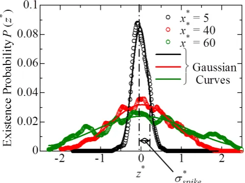
Figure 7 shows the spanwise existence probability distributions of the spikes at three downstream distances. The solid lines in the figure are the fitted Gaussian distribution curves for the calculated existence probability. Although there is some discrepancy be-tween the calculated distributions and the fitting curves, we can still say that the span-wise distribution of the existence probability almost follows the Gaussian shape. Basi-cally, a statistical random process of an event follows the Gaussian distribution. There-fore, the transport process of the high concentration spikes is a kind of random process similar to that of the plume.

The variations of the standard deviation σspike

∗ _{of the probability of spikes as a}

func-tion of the downstream distance are shown in Figure 8. While, for comparison, the diffusion width of the concentration plume σplume

∗ _{defined as the standard deviation of}

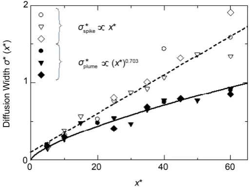
the spanwise mean concentration distribution of the plume is also calculated and shown in the figure. The PLIF images obtained by measurements repeated three times are used. This is done to enhance the reliability by having more data dots in the figure. The dashed line in Figure 8 is the approximate straight line to the standard deviations of the spikes by the least square method, while the solid line is the approximated curve to the standard deviations of the plume. It can be seen that the diffusion width of the concentra-tion plume increases as a power funcconcentra-tion of the downstream distance, corresponding to the result of Webster et al. [24]. Meanwhile, the diffusion width of the high concentra-tion spikes increases almost linearly with downstream distance, and the increase rate is larger than that of the plume width. Moreover, the diffusion widths of the spikes are larger than the corresponding plume widths. The reason is that the high concentration

Figure 8. Diffusion widths of high concentration spikes and plume versus downstream distance x*.

spikes are also extracted at the edge of the plume where there are low-concentration and large concentration gradients with the surrounding areas. To further clarify the difference between high concentration spikes and plume, the length scale, the ratio of mean concentration, and the turbulent diffusion coefficient were calculated, and the diffusion process of the spike is discussed.

4.3. Length Scale

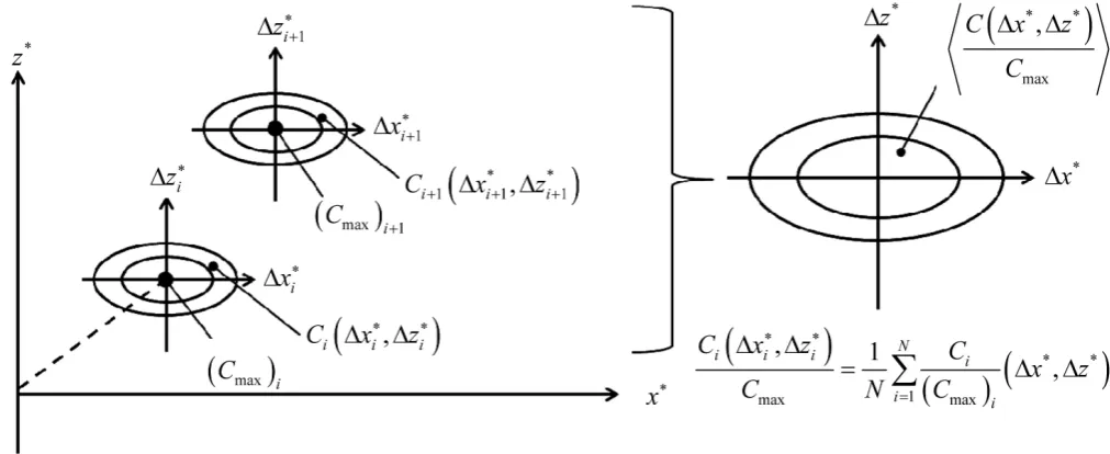
From Figure 6, it is difficult to understand the relationship between the concentration spikes and the increasing downstream distances. To provide quantitatively analysis of the relationship, the length scale of the high concentration spikes was calculated, in which the mean concentration of the spikes was involved. Figure 9 is a schematic dia-gram showing how to obtain the mean concentration distribution of spikes. Firstly, each high concentration spike on a binarized image was distinguished through a labe-ling technique and numbered in sequence as 1, 2,, ,i i+1,,N. Then, a new

coordi-nate system was established for each spike, with the origin located at the mass center of the spike; the horizontal axis and vertical axis respectively denoting the streamwise and spanwise distances from the mass center. Meanwhile, the maximum instantaneous concentration in each spike was extracted as Cmax and used to normalize the concentra-tion in the same spike. After normalizing concentraconcentra-tion Ci

(

)

∗ ∗

∆ ∆ _{in spike i with}

Figure 9. Calculation of mean concentration distribution in high concentration spikes.

Figure 10. Mean concentration distribution around high concentra-tion spikes at downstream distance of x* = 20 obtained by conditional average method.

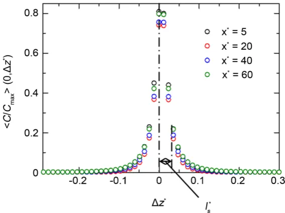
field in this experiment has a larger spanwise concentration gradient than that in the streamwise direction, which has great influences on the anisotropy of the distribution breadths in spanwise and streamwise direction. Focusing on Δx* = 0 extracts the span-wise mean concentration distribution through the resultant spike center, which com-bined with the results from other streamwise locations, is shown in Figure 11.

It is obvious that the profiles of the four streamwise locations coincide and the span-wise average length scale of the high concentration spike ls

∗_{, calculated as the standard}

deviation of the profile, is around 0.03 and independent of streamwise distances. The reason why ls

∗ _{remains constant instead of increasing downstream can be understood}

inversely: according to the conditional sampling technique, a spike is extracted based on the relatively high concentration and large concentration gradient values, which means that usually, a spike disappears when the concentration in the spike is diluted and diffused to the surroundings by molecular diffusion. Generally, the length scale, in which the mean concentration of the diffusing plume is involved, becomes bigger with progress of the diffusion of the plume concentration. Accordingly, larger scale spikes hardly exist and the average length scale of the spike is constant instead of increasing downstream. Moreover, the spanwise integral scale of eddies l* obtained by integration of the spanwise two-point correlation coefficient is found to be 0.3, larger than ls

∗

here. The length scale of the plume compared with the eddy’s length scale relates to the diffusion process. Yee and Wilson [25] investigated the action of eddies of length scale l on the plume in accordance with the relative sizes of l with respect to the length scale of the diffusing plume σr which corresponds to the standard deviation of the average in-stantaneous concentration distribution of the plume. They reported that, when l > σr, eddies of this size resulted in large-scale meandering of the instantaneous plume

centroid, and the concentration in the meandering plume hardly changed. By analogy, the relative scale of the turbulent eddies with respect to the length scale, calculated from the average concentration distribution of the spike, determines the diffusion process of the spike. For l* larger than ls

∗_{, the movement of the spike shows the meandering}

mo-tion resulting from the large scale acmo-tion of the turbulent eddy, and the diffusion inside the spike is insignificant. This may explain why the formed high concentration spikes shifts downstream with the internal concentration seldom changing.

4.4. Mean Concentration Ratio

The above section shows that the diffusivity of the inner concentration allows us to discuss the diffusion process. This section calculates the mean concentration ratio of the spikes to the plume, and investigates the diffusivity of the concentration inside the spikes. The mean concentration and the ratio of mean concentration are respectively defined by Equation (4) and Equation (5).

( )

_{( )}

( )

( )

(

₍

)

₎

C z C P

N z P P P δ ς =  =  =  ₌ 

∑

. (4)

( )

_{( )}

( )

plume

C z r z

C z

= _{. (5)}

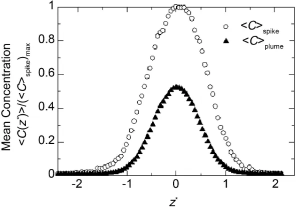
where, Nc denotes the total number of recognized spikes for a fixed z*; PC is binarized data indicating the existence of the high concentration spikes; ζ is an indicator function. Figure 12 gives the spanwise mean concentration distribution of the spikes and the

plume at x* = 20 for example. The mean concentration distributions are normalized by the maximum concentration in the spikes. As can be seen from Figure 12, the spanwise distribution shape of mean concentration for the spikes and plume are similar, both approximately following the Gaussian distribution. Considering that the spanwise mean concentration distribution matches Gaussian distribution when the mass is dis-tributed as random walk [26], it is inferred that the concentration distribution in the high concentration spikes is based on random walk.

Figure 13 shows the mean concentration ratio at each measurement position. This figure plots the ratios only for one spanwise side because the mean concentration ratio distributions are line-symmetric with respect to z* = 0. Comparing the two distribu-tions, the mean concentration ratio and the mean concentration of the plume, it seems that the ratio distribution continues increasing to the area where the mean concentra-tion of the plume is approximately zero. Inevitably, the mean concentraconcentra-tion ratio ex-ceeds one because the mean concentration of the high concentration spikes extracted as the areas with high concentration in the plume is larger than that of the plume. In addi-tion, the ratio should be constant with spanwise distance when the declines of concen-tration in the plume and the spike are the same, as is the case when they move the same distance in the spanwise direction due to diffusion phenomena. The result shows that the mean concentration ratio increases with spanwise distance, which means that the decline rate of concentration in the plume is larger than that in the high concentration spike with the same distance in spanwise direction. Therefore, the high concentration spike moves to the spanwise direction with low diffusivity of the internal concentration compared to the concentration plume, and the gap in diffusivity continues increasing to the edge of the concentration plume.

4.5. Apparent Diffusion Coefficient

We consider that there are two types of diffusivity of concentration in turbulent mass diffusion: one is the internal diffusivity of internal concentration with the travel dis-tance, and the other is the external diffusivity relating to the transport of the concentra-tion in a turbulent flow. To discuss the external diffusivity, the apparent diffusion coef-ficient is calculated in this section. The apparent diffusion coefcoef-ficient can be unders-tood as the magnitude of concentration flux divided by the local mean concentration gradient. Apparent diffusion coefficients in spanwise direction for plume and spikes are respectively calculated by Equation (6) and Equation (7) as follows,

( )

₍

₎

z

w C K

C z

′ ′ − =

∂ ∂ . (6)

( )

( )

(

)

spike *

spike

C z

w C P

K

C z

δ

′ ′ − =

∂ ∂ . (7)

where w' (=w − W>) denotes the spanwise velocity fluctuation, calculated from span-wise instantaneous velocity w and time-average spanspan-wise velocity <W>. Apparent dif-fusion coefficient for the plume (Kz)plume have the same physical meaning of the turbu-lent diffusion coefficient. In contrast with this, as the definition formula (7) for the ap-parent diffusion coefficient (Kz)spike includes the probability function δ(Pc), the value is affected by the local generation and disappearance of the spikes. Therefore, the appar-ent diffusion coefficiappar-ent of the spikes is the useful measure to describe the behavior of the spikes appearing in the outer edge of the plume but its meaning is different from the conventional turbulent diffusion coefficient. The calculated spanwise coefficient is shown in Figure 14 for non-negative spanwise locations along with the linear approx-imation of coefficients of spikes shown by the solid lines.

As is indicated, the apparent diffusion coefficient of the plume (Kz)plume is constant, independent of both the streamwise and spanwise distances, which implies that the as-sumption of homogeneous turbulent flow in our experiment is reasonable. However, unlike the coefficient of plume, (Kz)spike increases linearly with spanwise distance. Our analysis shows that the concentration flux driven by spanwise concentration gradient in the spike is more and more dominant as spanwise distance increases, compared with the concentration flux driven by spanwise concentration gradient in the plume. Also, there is a strong correlation between the spanwise velocity fluctuation and the concen-tration fluctuation. Actually, in a homogeneous turbulent flow, the high concenconcen-tration fluctuation has a large velocity fluctuation and the relationship between the concentra-tion and velocity fluctuaconcentra-tions is linear, as was reported by [27] [28]. From the mean concentration ratio, it is found that there is a gap between the mean concentrations of the spikes and plume, which means that the average concentration fluctuation of the spikes based on the mean concentration of the plume increases with the spanwise dis-tance. Based on the linear relationship between the concentration fluctuation and ve-locity fluctuation, the average veve-locity fluctuation of the spikes increases with the span-wise distance. This increase leads to an increase of the apparent diffusion coefficient of the spikes. Moreover, comparison of the linear approximations at different streamwise distances reveals a decreasing slope of the fitted line towards an increasing streamwise distance. The cause of this is considered to be that the concentration fluctuation is re-duced as the concentration approaches spatial homogeneity and thus the concentration flux decreases. Consequently, it can be seen that the diffusion process of the spikes dif-fers from that of the plume.

4.6. The Diffusion Theory of the High Concentration Spikes

in-stantaneous plume in meandering motions hardly change with the travel distance of the plume, and an increase of the length scale σr is caused when l ≈ σr. Therefore, there are four factors related to the diffusion process of the concentration plume diffusing in a turbulent flow: diffusion time, diffusion width, length scale, and the diffusivity of the internal concentration of the plume.

We cannot confirm the meandering motions of the diffusing plume in Figure 5, and suppose that a large part of the diffusion of the plume is strongly dominated by relative diffusion, based on the relationship between the diffusion time of the plume and the time integral scale of the turbulent flow. On the other hand, the calculated scalar statis-tics of the high concentration spikes have the same properties of meandering diffusion. The diffusion width of the high concentration spikes increases linearly with the down-stream distance as is shown in Figure 8. Figure 11 shows that the average length scale of the high concentration spikes keeps constant for downstream distance and is smaller than the length scale of the eddies. In addition, from the result of Figure 13, it is firmed that the high concentration spike has a lower apparent diffusivity of inner con-centration while moving in turbulent flow, compared with that of a plume dominated by relative diffusion. Consequently, it is concluded that the diffusion of a high concen-tration spike is dominated by meandering diffusion regardless of the diffusion process of the plume. The aggregation diffusion of the spikes is considered to be reflected in the combination of a high concentration spike dominated by a meandering diffusion. This may be the reason why diffusion width increases linearly for the downstream distance. Moreover, the number of spikes per unit of area increases with increasing downstream distance, as shown in Figure 6. Accordingly, neither the number nor the inner concen-tration of the high concenconcen-tration spikes extracted from the concenconcen-tration plume follows the conservation law which the plume diffusion satisfies, and this is the major differ-ence between the spike and the plume.

To reduce the damage from pollutant diffusion it is important to predict the diffu-sion of not only the mean concentration but also the concentration fluctuation. It is concluded that the large concentration fluctuation occurring at any position in a turbu-lent flow is greatly affected by meandering diffusion. This knowledge is expected to en-hance the accuracy of diffusion prediction of concentration fluctuation.

5. Conclusions

This paper focuses on the high concentration spike formed by turbulent structures, and we investigate their diffusion process from the viewpoint of the difference with the concentration plume.

As regards the average length scale of the spikes, it is found to be constant for the downstream distance and smaller than the integral scale of eddies, which differs from the character of the concentration plume. The turbulent diffusion coefficient of the spikes is proportional to the spanwise distance, while that of the plume is constant.

From all the results, we conclude that the diffusion process of a high concentration spike is dominated by the meandering diffusion consistently in a turbulent flow and differs from that of the plume. This knowledge is expected to help with the accurate diffusion prediction of concentration fluctuation.

References

[1] Takemura, T., et al. (2011) A Numerical Simulation of Global Transport of Atmospheric Particles Emitted from the Fukushima Daiichi Nuclear Power Plant. SOLA, 7, 101-104.

http://www.jstage.jst.go.jp/browse/sola https://doi.org/10.2151/sola.2011-026

[2] Terada, H. and Chino, M. (2008) Development of an Atmospheric Dispersion Model for Accidental Discharge of Radionuclides with the Function of Simultaneous Prediction for Multiple Domains and Its Evaluation by Application to the Chernobyl Nuclear Accident.

Journal of Nuclear Science and Technology, 45, 920-931.

https://doi.org/10.1080/18811248.2008.9711493

[3] Chino, M., Nakamura, H., Nagai, H., Terada, H., Katata, G. and Yamazawa, H. (2011) Pre-liminary Estimation of Release Amounts of 131_{I and} 137_{Cs Accidentally Discharged from the}

Fulushima Daiichi Nuclear Power Plant into the Atmosphere. Journal of Nuclear Science and Technology, 48, 1129-1134. https://doi.org/10.1080/18811248.2011.9711799

[4] Taylor, G.I. (1921) Diffusion by Continuous Movement. Proceedings of the Royal Society A, 20, 196-211.

[5] Richardson, L.F. (1926) Atmospheric Diffusion Shown on a Distance-Neighbor Graph.

Proceedings of the Royal Society A, 110, 709-737. https://doi.org/10.1098/rspa.1926.0043

[6] Brown, R.J. and Bilger, R.W. (1996) An Experiment Study of a Reactive Plume in Grid Turbulence. Journal of Fluid Mechanics, 312, 373-407.

https://doi.org/10.1017/S0022112096002054

[7] Lemoine, F., Wolff, M. and Lebouche, M. (1997) Experimental Investigation of Mass Transfer in a Grid-Generated Turbulent Flow Using Combined Optical Methods. Interna-tional Journal of Heat and Mass Transfer, 40, 3255-3266.

https://doi.org/10.1016/S0017-9310(96)00385-7

[8] Lemoine, F., Antoine, Y. and Lebouche, M. (2000) Some Experimental Investigations on the Concentration Variance and Its Dissipation Rate in a Grid Generated Turbulent Flow. In-ternational Journal of Heat and Mass Transfer, 43, 1187-1199.

https://doi.org/10.1016/S0017-9310(99)00204-5

[9] Nagata, K., Suzuki, H., Sakai, Y., Hayase, T. and Kubo, T. (2008) Direct Numerical Simula-tion of Turbulent Mixing in Grid-Generated Turbulence. Physica Scripta, 132, 1-5.

[10] Antonia, R.A., Chambers, A.J., Britz, D. and Browne, L.W.B. (1986) Organized Structure in a Turbulent Plane Jet: Topology and Contribution to Momentum and Heat Transport.

Journal of Fluid Mechanics, 172, 211-229. https://doi.org/10.1017/S0022112086001714

[11] Buch, K.A. and Dahm, W.J.A. (1996) Experimental Study of the Fine-Scale Structure of Conserved Scalar Mixing in Turbulent Shear Flows. Journal of Fluid Mechanics, 317, 21-71.

[12] Tong, C. and Warhaft, Z. (1994) On Passive Scalar Derivative Statistics in Grid Turbulence.

Physics of Fluids, 6, 2165-2176. https://doi.org/10.1063/1.868219

[13] Holzer, M. and Siggia, E.D. (1994) Turbulent Mixing of a Passive Scalar. Physics of Fluids, 6, 1820-1837. https://doi.org/10.1063/1.868243

[14] Webster, D.R., Volyanskyy, K.Y. and Weissburg, M.J. (2011) Sensory-Mediated Tracking Behavior in Turbulent Chemical Plumes. Proceedings of the 7th International Symposium on TSFP,Ottawa, 28-31 July 2011, 1-6.

[15] Page, J.L., Dickman, B.D., Webster, D.R. and Weissburg, M.J. (2011) Getting Ahead: Con-text-Dependent Responses to Odorant Filaments Drive Along-Stream Progress during Odor Tracking in Blue Crabs. Journal of Experimental Biology, 214, 1498-1512.

https://doi.org/10.1242/jeb.049312

[16] Endo, M., Tsukahara, T. and Yasuo, K. (2015) Relationship between Diffusing-Material Lumps and Organized Structures in Turbulent Flow. Proceedings of the 5th International AJK Joint Fluids Engineering Conference,Seoul, 26-31 July 2015, 1747-1753.

[17] Hu, H., Saga, T., Kobayashi, T. and Taniguchi, N. (2002) Simultaneous Velocity and Con-centration Measurements of a Turbulent Jet Mixing Flow. Annals of the New York Acade-my of Sciences, 972, 254-259. https://doi.org/10.1111/j.1749-6632.2002.tb04581.x

[18] Diez, F.J., Bernal, L.P. and Faeth, G.M. (2005) PLIF and PIV Measurements of the Self-Preserving Structure of Steady Round Buoyant Turbulent Plumes in Crossflow. Inter-national Journal of Heat and Fluid Flow, 26, 873-882.

https://doi.org/10.1016/j.ijheatfluidflow.2005.10.003

[19] Janzen, J.G., Herlina, H., Jirka, G.H., Schulz, H.E. and Gulliver, J.S. (2010) Estimation of Mass Transfer Velocity Based on Measured Turbulence Parameters. AIChE, 56, 2005-2017. [20] Pope, S.B. (2000) Turbulent Flows. Cambridge University Press, Cambridge, 305-308. [21] Cryer, J.D. (1983) Time Series Analysis. Duxbury Press, Boston, 1-487.

[22] Kosugi, K., Makita, H. and Haniu, H. (2014) Experiment Investigation on Turbulent Diffu-sion Phenomena of Meandering Plume in the Quasi-Isotropic Turbulent Field (Variation of Mean Concentration Properties for Turbulent Reynolds Numbers). Transactions of the JSME, 80, 1-14. (In Japanese)

[23] Hanna, S.R. (1981) Turbulent Energy and Lagrangian Time Scales in the Planetary Boun-dary Layer. Proceedings of the 5th Symposium on Turbulence, Diffusion, and Air Pollution, Atlanta, 9-13 March 1981, 61-62.

[24] Webster, D.R., Rahman, S. and Dasi, L.P. (2003) Laser-Induced Fluorescence Measure-ments of a Turbulent Plume. Journal of Engineering Mechanics, 129, 1130-1137.

https://doi.org/10.1061/(ASCE)0733-9399(2003)129:10(1130)

[25] Yee, E. and Wilson, D.J. (2000) A Comparison of the Detailed Structure in Dispersing Tracer Plumes Measured in Grid-Generated Turbulence with a Meandering Plume Model Incorporating Internal Fluctuations. Boundary-Layer Meteorology, 94, 253-296.

https://doi.org/10.1023/A:1002457317568

[26] Metzler, R. and Klafter, J. (2000) The Random Walk’s Guide to Anomalous Diffusion: A Fractional Dynamics Approach. Physics Reports, 339, 1-77.

https://doi.org/10.1016/S0370-1573(00)00070-3

[27] Pope, S.B. (1985) PDF Methods for Turbulent Reactive Flows. Progress in Energy and Combustion Science, 11, 119-192. https://doi.org/10.1016/0360-1285(85)90002-4

[28] Brethouwer, G. and Nieuwstadt, F.T.M. (2001) DNS of Mixing and Reaction of Two Species in a Turbulent Channel Flow: A Validation of the Conditional Moment Closure. Flow,

Submit or recommend next manuscript to SCIRP and we will provide best service for you:

Accepting pre-submission inquiries through Email, Facebook, LinkedIn, Twitter, etc. A wide selection of journals (inclusive of 9 subjects, more than 200 journals)

Providing 24-hour high-quality service User-friendly online submission system Fair and swift peer-review system

Efficient typesetting and proofreading procedure

Display of the result of downloads and visits, as well as the number of cited articles Maximum dissemination of your research work

Submit your manuscript at: http://papersubmission.scirp.org/