BIROn - Birkbeck Institutional Research Online
Marx, D. and Razgon, Igor (2014) Fixed-parameter tractability of multicut
parameterized by the size of the cutset. SIAM Journal on Computing 43
(2), pp. 355-388. ISSN 0097-5397.
Downloaded from:
Usage Guidelines:
Fixed-parameter tractability of multicut parameterized by the size
of the cutset
∗D´aniel Marx† Igor Razgon‡
Abstract
Given an undirected graphG, a collection{(s1, t1), . . . ,(sk, tk)} of pairs of vertices, and an integer p, the Edge Multicut problem ask if there is a set S of at most p edges such that the removal of S disconnects every si from the corresponding ti. Vertex Multicut is the analogous problem whereS is a set of at mostpvertices. Our main result is that both problems can be solved in time 2O(p3)·nO(1), i.e., fixed-parameter tractable parameterized by the sizepof
the cutset in the solution. By contrast, it is unlikely that an algorithm with running time of the form f(p)·nO(1) exists for the directed version of the problem, as we show it to be W[1]-hard
parameterized by the size of the cutset.
1
Introduction
From the classical results of Ford and Fulkerson on minimum s−t cuts [16] to the more recent
O(√logn)-approximation algorithms for sparsest cut problems [35, 1, 14], the study of cut and separation problems have a deep and rich theory. One well-studied problem in this area is the
Edge Multicut problem: given a graph G and pairs of vertices (s1, t1), . . ., (sk, tk), remove
a minimum set of edges such that every si is disconnected from its corresponding ti for every
1 ≤ i ≤ k. For k = 1, Edge Multicut is the classical s−t cut problem and can be solved
in polynomial time. For k = 2, Edge Multicut remains polynomial-time solvable [37], but it
becomes NP-hard for every fixed k ≥ 3 [11]. Edge Multicut can be approximated within a
factor ofO(logk) in polynomial time [17] (even in the weighted case where the goal is to minimize the total weight of the removed edges). However, under the Unique Games Conjecture of Khot [24], no constant factor approximation is possible [7]. One can analogously define the Vertex
Multicut problem, where the task is to remove a minimum set of vertices. An easy reduction
shows that the vertex version is more general than the edge version.
Using brute force, one can decide in timenO(p) if a solution of size at mostpexists. Our main result is a more efficient exact algorithm for small values of p (the O∗ notation hides factors that are polynomial in the input size):
Theorem 1.1. Given an instance of Vertex Multicut or Edge Multicutand an integer p, one can find in time O∗(2O(p3)) a solution of size p, if such a solution exists.
That is, we prove thatVertex MulticutandEdge Multicutare fixed-parameter tractable
parameterized by the size pof the solution, resolving a very challenging open question in the area
∗
A preliminary version of the paper was presented at STOC 2011 [28].
†
Institute for Computer Science and Control, Hungarian Academy of Sciences (MTA SZTAKI),[email protected] ‡
Department of Computer Science and Information Systems, Birkbeck, University of London.
of parameterized complexity. (Recall that a problem is fixed-parameter tractable (FPT) with a particular parameter p if it can be solved in time f(p)·nO(1), where f is an arbitrary computable
function depending only on p; see [13, 15, 30] for more background). The question was first asked explicitly perhaps in [25]; it has been restated more recently as an open problem in e.g., [20, 8]. Our result shows in particular that multicut is polynomial-time solvable if the size of the optimum solution isO(√3logn) (wheren is the input size).
One reason why multicut is a fundamental problem is that it is able to express several other
problems. It has been observed that a correlation clustering problem called Fuzzy Cluster
Editing can be reduced to (and in fact, equivalent with) Edge Multicut[3, 12, 2]. Our results
show thatFuzzy Cluster Editing is FPT parameterized by the editing cost, settling this open
problem discussed e.g., in [3].
Previous work. The fixed-parameter tractability of multicut and related problems has been thoroughly investigated in the literature. Edge Multicut is NP-hard on trees, but it is known
to be FPT, parameterized by the maximum number p of edges that can be deleted, and admits
a polynomial kernel [5, 21]. Multicut problems were studied in [20] for certain restricted classes
of graphs. For general graphs, Vertex Multicut is FPT if both p and and the number of
terminal pairs k are chosen as parameters (i.e, the problem can be solved in time f(p, k)·nO(1)
[26, 36, 19] for some functionf). The algorithm of Theorem 1.1 is superior to these result in the
sense that the running time depends polynomially on the number k of terminals pairs, and the
exponential dependence is restricted to the parameter p, the number of deletions. For the special case ofMultiway Cut(where terminals in a setT have to be pairwise separated form each other), algorithms with running time of the formf(p)·nO(1)were already known [26, 8, 19], but apparently these algorithms do not generalize in an easy way to multicut. An FPT 2-approximation algorithm was given in [27] forEdge Multicut: in time O∗(2O(plogp)), one can find a solution of size 2pif a solution of size p exists. There is no obvious FPT algorithm for the problem even on bounded-treewidth graphs, although one can obtain linear-time algorithms if the bounded-treewidth remains bounded after adding an edge siti for each terminal pair [18, 31]. A PTAS is known for bounded-degree
graphs of bounded treewidth [6].
Our techniques. The first two steps of our algorithm follows [27]. We start by an opening step that is fairly standard in the design of FPT algorithms. Instead of solving the originalVertex
Multicut problem, we solve the compression version of the problem, where the input contains
a solution W of size p+ 1, and the task is to find a solution of size p (if exists). A standard
argument called iterative compression [34, 23] shows that if the compression problem is FPT,
then the original problem is FPT. Alternatively, we can use the polynomial-time approximation algorithm of Gupta [22], which produces a solution W of size p2 if a solution of size p exists. In this case,O(p2) iterations of the compression algorithm gives a solution of sizep.
Next, as in [27], we try to reduce the compression problem to Almost 2SAT(deletek clauses
to make a 2-CNF formula satisfiable; also known as2CNF Deletion), which is known to be FPT
[33, ?, 32]. However, our 2SAT formulation is very different from the one in [27]: we introduce a single variable xv only for each vertex ofG, while in [27] there is a variable xv,w for every vertex
v ∈ V(G) and vertex w ∈ W of the initial solution. This simpler reduction to Almost 2SAT is correct only if the instance satisfies two quite special properties:
(1) every component ofG\W is adjacent to at most two vertices ofW (“has at most two legs”), and
to achieve property (1), we show by an analysis of cuts and performing appropriate branching
steps that the set W can be extended in such a way that every component has at most two legs
(Section 4). To achieve property (2), we describe a nontrivial way of sampling random subset of vertices such that if we remove this subset by a certain contraction operation (taking the torso of the graph), then without changing the solution, we get rid of the parts not reachable from W
with some positive probability (Section 3). This random sampling uses the concept of “important separators,” which was introduced in [26], and has been implicitly used in [9, 33, 8] in the design of parameterized algorithms. We consider the random sampling of important separators the main new technical idea of the paper. This technique and its generalizations have turned out to be useful for other problems as well [?, ?,?, ?, ?,?, ?] and we expect it to have further application in the future.
Directed graphs. Having resolved the fixed-parameter tractability ofVertex Multicut, the next obvious question is what happens on directed graphs. Note that for directed graphs, the edge and vertex versions are equivalent. In directed graphs, multicut becomes much harder to approx-imate: there is no polynomial-time 2log1−n-approximation for any > 0, unless NP⊆ ZPP [10]. From the fixed-parameter tractability point of view, the directed version of the problem received
particular attention because Directed Feedback Vertex Set or DFVS (delete p vertices to
make the graph acyclic) can be reduced toDirected Multicut. The fixed-parameter tractability of DFVS had been a longstanding open question in the area of parameterized complexity until it was solved by Chen et al. [9] recently. The main idea that led to the solution is that DFVS can
be reduced to a variant (in fact, special case) of Directed Multicut called Skew Multicut,
where the task is to break every path from si to tj for everyi > j. By showing that Skew
Mul-ticutis FPT parameterized by the size of the solution, Chen et al. [9] proved the fixed-parameter
tractability of DFVS. We show in Section 6 that, unlike Skew Multicut, the general Directed
Multicutproblem is unlikely to be FPT.
Theorem 1.2. Directed Multicutis W[1]-hard parameterized by the size p of the solution.
Independent and followup work. A preliminary version of this paper appeared in [28]; the current version contains essentially the same algorithm, but the terminology and organization of Section 5 were significantly changed. Independently from our work, Bousquet et al. [4] presented in the same volume a proof that Multicutis FPT parameterized by the sizep of the solution. The two algorithms have certain parts in common: both reduce the problem to the compression version and both ensure that we have to deal with components having only two legs. However, the main part of the two algorithms are substantially different: the current paper introduces the technique of random sampling of important separators and uses it to reduce the problem toAlmost 2SAT, while Bousquet et al. [4] uses an approach based on a series of problem-specific reductions to reduce the problem to 2SAT.
Subsequently to the first version of this paper, random sampling of important separators has been used in several other applications. For undirected graphs, the technique was used by Lok-shtanov and Ramanujan [?] to solve a parity version of Multiway Cut and by Chitnis et al. [?] to solve a homomorphism problem generalizing certain deletion problems. For directed graphs,
even though Directed Multicut is W[1]-hard parameterized by p (see Section 6), Chitnis et
al. [?] proved that the special case Directed Multiway Cut (Given a set T of terminals, break every directed path between two different terminals by removing at most pedges/vertices) is FPT parameterized byp. A consequence of this result is that Directed Multicutwithk= 2 is FPT parameterized bypis FPT. Kratsch et al. [?] proved thatDirected Multicuton directed acyclic
showing that Directed Multicut remains W[1]-hard parameterized byp even on DAGs.
How-ever, the complexity of Directed Multicut for k = 3 or with combined parameters k and p
remains an interesting open question.
Chitnis et al. [?] use the random sampling technique to show the fixed-parmeter tractability of
Directed Subset Feedback Vertex Set. They present an abstract framework in which this
technique can be used an improve the randomized selection and its analysis to obtain better success probability and improved running time.
A very different application of the technique is given by Lokshtanov and Marx [?] in the context of clustering problems. They study a family of clustering problems such as partitioning the vertices of an undirected graph into clusters of size at mostp such that at mostq edges leave each cluster. The problem boils down to being able to check whether a given vertex v is contained in such a cluster. It turns out that the random sampling of important separators technique can be used to show that this task (and therefore the original clustering problem) is FPT parameterized by q by reducing it to a knapsack-like problem.
2
Framework: compression, shadows, legs
Let G be an undirected graph and let T = {(s1, t1), . . . ,(sk, tk)} be a set of terminal pairs. We
say that a set S⊆V(G) of vertices is a multicutof (G,T) if there is no component1 ofG\S that
contains both si and ti for some 1≤ i≤k (note that it is allowed thatS contains si orti). The
central problem of the paper is the following:
Vertex Multicut
Input: A graphG, an integer p, and a setT of pairs of vertices ofG.
Output: A multicut of (G,T) of size at mostp
or “NO” if no such multicut exists.
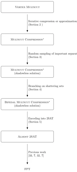
We prove the fixed-parameter tractability of Vertex Multicut by a series of reductions (see
Figure 1). First we argue that it is sufficient to solve an easiersolution compressionproblem. Then we present two reductions that modify the problem in such a way that it is sufficient to look for solutions that areshadowless and we can assume that the instance isbipedal. The last step of the proof is reducing this special variant of the problem to Almost 2SAT.
2.1 Compression
The first step in the proof of Theorem 1.1 is a standard technique in the design of parameterized
algorithms: we define and solve the compression problem, where it is assumed that the input
contains a feasible solution of size larger thanp. As this technique is standard (and in particular, we follow the approach of [27] for Edge Multicut), we keep this section short and informal.
Multicut Compression
Input: A graphG, an integer p,
a setT of pairs of vertices ofG, and a multicut W of (G,T).
Output: A multicut of (G,T) of size at mostp, or “NO” if no such multicut exists.
1Throughout this paper, when we refer to a component K of a graph, we consider the set of vertices of this
Vertex Multicut
Multicut Compression∗
Multicut Compression∗
(shadowless solution)
Bipedal Multicut Compression∗
(shadowless solution)
Almost 2SAT
FPT
Iterative compression or approximation (Section 2 )
Random sampling of important separators (Section 3)
Branching on shattering sets (Section 4)
Encoding into 2SAT (Section 5)
[image:6.612.143.415.76.678.2]Previous work [33,?, 32,?]
Our main technical contribution is showing that Multicut Compressionis FPT parameterized by pand |W|.
Lemma 2.1. Multicut Compression can be solved in time O∗(2O((p+log|W|)3+|W|log|W|)).
Intuitively, it is clear that proving Lemma 2.1 could be easier than proving that Vertex
Multicut is FPT: the extra input W can give us useful structural information about the graph
(and as |W| appears in the running time, a large W is also helpful). What’s not obvious is
how solving Multicut Compression gives us any help in the solution of the original Vertex
Multicutproblem. We sketch two methods.
Method 1. Let us use the polynomial-time approximation algorithm of Gupta [22] to find a multicutW of size at mostc·OPT2, wherecis a universal constant and OPT is the minimum size of a multicut. If |W| ≥c·p2, then we can safely answer “NO”, as there is no multicut of size at mostp. Otherwise, we run the algorithm of Lemma 2.1 for this set W to obtain a solution in time
O∗(2O((p+log|W|)3)=O∗(2O(p3)).
Method 2. The standard technique of iterative compression [34, 23] allows us to reduce
Vertex Multicut to at most |V(G)|instances of Multicut Compression with |W|=p+ 1.
This technique was used for the 2-approximation of Edge Multicut in [27] and its application
is analogous in our case. Let (G,T, p) be an instance of Vertex Multicut. Suppose that
V(G) = {v1, . . . , vn}, let Gi =G[{v1, . . . , vi}], and letTi be the subset ofT containing the pairs
with both endpoints inGi. One by one, we consider the instances (Gi,Ti, p) in ascending order of
i, and for each instance we find a solutionSi of size at most p. We start with S0 = ∅. For some
i >0, we compute Si provided that Si−1 is already known. Observe that Si−1∪ {vi}is a multicut
of size at most p+ 1 for (Gi,Ti). Thus we can use the algorithm for Multicut Compression, which either returns a multicut Si of (Gi,Ti) having size at most p or returns “NO”. In the first
case, we can continue the iteration withi+ 1. In the second case, we know that there is no multicut of sizepfor (G,T) (as there is no such multicut even for (Gi,Ti)), and hence we can return “NO”.
Both methods result in O∗(2O(p3)) time algorithms. However, we feel it important to mention both approaches, as improvements in Lemma 2.1 might have different effects on the two methods. It will be convenient to work with a slightly modified version of the compression problem. We say that a set S ⊆V(G) is a multiway cutof W ⊆V(G) if every component of G\S contains at most one vertex ofW.
Multicut Compression∗
Input: A graphG, an integer p,
a setT of pairs of vertices ofG, and a multicut W of (G,T).
Output: A setS of size at mostp such that (1) S is multicut of (G,T), (2) S∩W =∅, and
(3) S is a multiway cut of W
or “NO” if no such setS exists.
That is,Multicut Compression∗has two additional constraints on the solutionS. In Sections 4– 5, we prove that this problem is FPT:
Figure 2: The shadow of S consists of the three sets C1,C2,C3.
It is not difficult to reduce Multicut Compression toMulticut Compression∗ (an
anal-ogous reduction was done in [27] for the the edge case). We briefly sketch such a reduction. In order to solve an instance (G,T, W, p) ofMulticut Compression, we first guess the intersection
X of the multicutW given in the input and the solution S we are looking for. This guess results in at mostPp
i=1 |W|
i
branches; in each branch, we remove the vertices of X from Gand decrease
p by |X|. Thus in the following, we can restrict our attention to solutions disjoint fromW. Next, we branch on all possible partitions (W1, . . . , Wt) ofW, contract each Wi into a single vertex, and
solve Multicut Compression∗ on the resulting instance (G0,T0, W0, p0). One of the partitions (W1, . . . , Wt) corresponds to the way the solutionS partitions W into connected components, and
in this caseS is a multiway cut ofW0 inG0. Thus if the originalMulticut Compressioninstance has a solutionS, then it is a solution of one of the constructedMulticut Compression∗instances. Conversely, any solution of the constructed instances is a solution of the original instance. As the number of partitions ofW can be bounded by |W|O(|W|), the running time claimed in Lemma 2.1
follows from Lemma 2.2. Thus in the rest of the paper, it is sufficient to prove Lemma 2.2 to obtain the main result, i.e., Theorem 1.1. Thus proving Lemma 2.2 implies the main result Theorem 1.1.
2.2 Shadows
An important step in our algorithm forMulticut(and in further applications of the randomized sampling of important separators method) is to argue about solutions that are “shadowless” in the sense defined below. Intuitively, we imagine the vertices inW as light sources, light spreads on the edges, andS blocks the light (see Figure 2).
Definition 2.3. Let I = (G,T, W, p) be an instance of the Multicut Compression∗ problem,
and letS be a solution forI. Theshadow of the setS is the set of vertices not reachable from any vertex ofW in G\S. We say that the solutionS is shadowlessif the shadow is empty, i.e., G\S
has exactly |W|components.
In Section 3, we present a randomized algorithm that modifies the instance such that if a solution exists, then it makes the solution shadowless with positive probability. The algorithm is based on a randomized contraction of sets defined by “important separators”; we review this concept in Section 3.3. The algorithm can be derandomized to obtain the following lemma:
Lemma 2.4 (shadowless reduction). Given an instanceI of the Multicut Compression∗
prob-lem, we can construct in time O∗(2O(p3)) a set of t = 2O(p3)logn instances I1, . . ., It, each with
the same parameter p as I, such that
1. Any solution of Ii for any1≤i≤t is a solution of I.
2. If I has a solution, then Ii has a shadowless solution for at least one 1≤i≤t.
Thus Lemma 2.4 allows us to reduce the Multicut Compression∗ problem into a variant
where the task is to find a shadowless solution.
2.3 Components and legs
In order to find a shadowless solution for a Multicut Compression∗ instance, the problem is
Figure 3: An instance with 7 components. The strong circles are the vertices of W, the numbers show the number of legs for each component.
Definition 2.5. Given an instance (G,T, W, p) of Multicut Compression∗, we say that a
componentC of G\W has `-legsif C is adjacent with `vertices of W (see Figure 3). We say that
a Multicut Compression∗ instance isbipedalif every component ofG\W has at most two legs;
Bipedal Multicut Compression∗ is the problem restricted to such instances.
The transformation presented in Section 4 reduces Multicut Compression∗ to a bounded
number of bipedal instances.
Lemma 2.6 (bipedal reduction). Given an instanceI of the Multicut Compression∗ problem
with parameter p, in time O∗(2O((p+log|W|)3)) we can either solve this instance or construct a set of
t= 2O(p+log|W|)3 instancesI1,. . .,It, of Bipedal Multicut Compression∗ each with parameter
at mostp, such that
1. Any solution of Ii for any1≤i≤t is a solution of I.
2. If I has a shadowless solution, then Ii has a shadowless solution for at least one 1≤i≤t.
Finally, in Section 5, we show how this solution can be found by a quite intuitive reduction to
an FPT problem Almost 2SAT.
Lemma 2.7. Let I = (G,T, W, p) be an instance of Bipedal Multicut Compression∗ that
has a shadowless solution S of size at most p. In time O∗(4p), we can find a (not necessarily
shadowless) solutionS0.
Combining Lemmas 2.4–2.7 allows us to prove Lemma 2.2 and therefore to solve Vertex
Multicut.
Proof (of Lemma 2.2). Let us apply the Algorithm of Lemma 2.4 to an instance I = (G,T, W, p)
of Multicut Compression∗. This algorithm takes time O∗(2O(p3)) and producest= 2O(p3)logn
instancesIi of theMulticut Compression∗ problem, each with parameter at mostp, so that the original instanceI has a solution if and only if one of these t instances has ashadowless solution. Moreover a (not necessarily shadowless) solution of any of these instances is also a solution of the orginal instance.
Apply to each instance Ii the algorithm of Lemma 2.6, which in time O∗(2O((p+log|W|)
3)
) either returns an answer or produces 2O((p+log|W|)3) instancesIi,j, each with parameter at mostp, of the
Bipedal Multicut Compression∗ problem such that Ii has a shadowless solution if and only if
at least oneIi,j has a shadowless solution. Moreover a (not necessarily shadowless) solution of any
new instanceIi,j is also a solution of Ii.
Combining the above two steps, we conclude that in timeO∗(2O((p+log|W|)3)) the algorithm pro-duces 2O((p+log|W|)3)logninstances of theBipedal Multicut Compression∗ problem such that the original instanceI has a solution if and only if at least one of the these 2O((p+log|W|)3)logn in-stances has a shadowless solution. Moreover a (not necessarily shadowless) solution of any instance
Ii,j is also a solution of I.
Finally, we apply to each resulting instance Ii,j of the Bipedal Multicut Compression∗
Figure 4: The torso operation on the graph Gwith a setC of 6 vertices.
returns “NO” for all the instances, this means that no one of them has a shadowless solution. It follows that the original instance does not have a solution either. Taking into account that the algorithm of Lemma 2.7 takes time O∗(4p), processing of 2O((p+log|W|)3)logn instances takes time
O∗(2O((p+log|W|)3)). Consequently, the instance I of the Multicut Compression∗ problem can be solved in time O∗(2O((p+log|W|)3)).
3
Making the solution shadowless
The purpose of this section is to reduce solvingMulticut Compression∗ to finding a shadowless
solution. We present a randomized transformation that, given an instance having a solution,
modifies the instance in such a way that the new instance has ashadowlesssolution with probability 2−O(p3). More precisely:
Lemma 3.1. Given an instanceI of the Multicut Compression∗ problem, we can construct in
time O∗(2O(p)) an instanceI0 with the same parameterp asI such that 1. Any solution of I0 is a solution of I.
2. If I has a solution, then I0 has ashadowless solution with probability 2−O(p3).
This means that if I has a solution, then by invoking Lemma 3.1 2O(p3) times, with constant probability at least one of the instances has a shadowless solution. Thus if we are able to solve the problem with the assumption that a shadowless solution exists, then this way we can get a solution for I with constant probability. The main result of this section is a derandomized version of this transformation (Lemma 2.4).
The main idea in the proof of Lemma 3.1 is to try to randomly guess a setZ whose removal does not change the instance substantially, but makes the instance shadowless. Section 3.1 introduces the torso operation, which is used to remove the setZ, and states what properties the setZ needs to satisfy. The construction ofZ is based on the observation that the solution can be characterized by a “closest set” and we need to locate the boundary of such a set (Section 3.2). We develop a randomized algorithm for this purpose in Sections 3.3–3.6. The algorithm uses the notion of important separators; Section 3.3 reviews this concept and shows why it is relevant for our problem. Sections 3.4–3.5 describe and analyze the randomized selection process. Section 3.6 shows how the random selection can be derandomized to obtain the deterministic version, Lemma 2.4.
3.1 Torsos and shadowless solutions
The randomized transformation can be conveniently described using the operation of taking the
torsoof a graph.
Definition 3.2. Let G be a graph and C ⊆V(G). The graph torso(G, C) has vertex set C and two vertices a, b ∈ C are adjacent if {a, b} ∈E(G) or there is a path P in G connecting a and b
whose internal vertices are not in C.
Proposition 3.3. Let C ⊆ V(G) be a set of vertices in G and let a, b ∈ C two vertices. A set
S ⊆C separates vertices aand b in torso(G, C) if and only if S separates these vertices in G. Proof. Let P be a path connecting a and b in G and suppose that P is disjoint from the set S. The path P contains vertices from C and from V(G)\C. If u, v ∈C are two vertices such that every vertex of P between u and v is from V(G)\C, then by definition there is an edge uv in
torso(G, C). Using these edges, we can modify P to obtain a path P0 that connects a and b in
torso(G, C) and avoids S.
Conversely, suppose thatP is a path connectingaandbin the graphtorso(G, C) and it avoids
S ⊆ C. If P uses an edge uv that is not present in G, then this means that there is a path
connecting u and v whose internal vertices are not in C. Using these paths, we can modify P to obtain a pathP0 that uses only the edges of G. SinceS⊆C, the new vertices on the path are not inS, i.e., P0 avoids S as well.
Let I = (G, W,T, p) be an arbitrary instance of Multicut Compression∗. Given a set
Z ⊆V(G)\W of vertices, thereduced instanceI/Z = (G0, W,T0, p) is defined the following way: 1. The graph G0 is torso(G, V(G)\Z).
2. For everyv∈V(G), letφ(v) =N(C) ifvbelongs to componentCofG[Z], and letφ(v) ={v} ifv 6∈ Z. The set T0 is obtained by by replacing every pair (x, y) ∈T with the set of pairs {(x0, y0)|x0 ∈φ(x), y0 ∈φ(y)}.
The main observation is that if we perform this torso operation for aZ that is sufficiently large to cover the shadow of a hypothetical solution S and sufficiently small to be disjoint from S, then
S becomes a shadowless solution of I/Z. Furthermore, the torso operation is “safe” in the sense that it does not make the problem easier, i.e, does not create new solutions.
Lemma 3.4. Let I = (G,T, W, p) be an instance of Multicut Compression∗ and let Z ⊆
V(G)\W be a set of vertices.
(1) Every solution of I/Z is a solution of I.
(2) If I has a solution S such that Z covers the shadow and Z∩S =∅, then S is a shadowless solution of I/Z.
Proof. LetGand G0=torso(G, V(G)\Z) be the graphs in instancesI andI/Z, respectively. To prove the first statement, we show that ifS0 ⊆V(G0) is a solution ofI/Z, thenS0 is a solution ofI
as well. Suppose that some pair (x, y) of I is not separated byS0. LetP be a path inG\S0 going fromx toy. Letx0 andy0 be the first and last vertex of P not in Z, respectively, and letP0 be the subpath ofP fromx0 toy0. (Note thatP cannot be fully contained inZ, as it contains at least one vertex of the multicut W.) By the way I/Z is defined, (x0, y0) is a pair in I/Z, hence S0 separates
x0 and y0 in G0 = torso(G, C). Using Prop. 3.3 with C =V(G)\Z, we get thatS0 separatesx0
and y0 inG, which is in contradiction with the existence of the pathP. A similar argument shows that there is no path in G\S0 that connects two vertices ofW.
For the second statement, suppose that Sis a solution ofI withS∩Z =∅. Let us show thatS
is a solution of I/Z as well. Suppose thatS does not separatex0 and y0 inG0 for some pair (x0, y0) of I/Z. Using Prop. 3.3 withC =V(G)\Z, we get thatS0 does not separate x0 and y0 in G, i.e., there is anx0−y0 pathP inG\S. By the way the pairs inI/Z were defined, there is a pair (x, y) of I and there is an x−x0 pathP1 such that x0 is the only vertex of P1 not in Z, and there is a
y−y0 pathP2 such thaty0 is the only vertex ofP2 not in Z. Clearly, these paths are disjoint form
S. Therefore, the concatenation of P1,P, P2 is an x−y path in G\S, contradicting thatS is a
To see thatSis shadowless inG0, consider a vertexvofG0\S. Asv6∈Z is not in the shadow of the solutionS ofI, there is a pathP inG\S going fromvto a vertexw∈W. Again by Prop. 3.3, this means that there is av−w path inG0\S as well, which means thatv is not in the shadow of the solutionS ofI0.
3.2 Closest sets
Lemma 3.4 shows that in order to reduce the Multicut Compression∗ problem to finding a
shadowless solution, all we need is a setZ that covers the shadow of a hypothetical solutionS, but disjoint from S itself. It is not obvious how this observation is of any help: it seems that there is no way of constructing such a set without actually knowing a solutionS. Nevertheless, we present a randomized procedure that constructs such a set with non-negligible probability.
The main idea of the randomized procedure is that a solution of a Multicut Compression∗
instance can be characterized by the set of vertices reachable fromW, and we can assume that this set has the property that it cannot be made smaller without increasing the size of the boundary. The following definition formalizes this property:
Definition 3.5. Let G be an undirected graph and let W ⊆V(G) be a subset of vertices. We say that a set R⊇W is a W-closest setif there is no R0 ⊂R withR0⊇W and |N(R0)| ≤ |N(R)|.
The main technical idea of the paper is the following randomized procedure, which, in some sense, finds the boundary of a closest set. Note that this statement could be of independent interest, as it is about closest sets in general and contains nothing specific to multicut problems.
Theorem 3.6 (random sampling). There is a randomized algorithm RandomSet(G, W, p) that, given a graph G, a set W ⊆V(G), and an integer p, produces a set Z ⊆V(G)\W such that the following holds. For every W-closest set R with |N(R)| ≤p, the probability that the following two events both occur is at least 2−O(p3):
1. N(R)∩Z =∅, and 2. V(G)\(R∪N(R))⊆Z.
That is, the two events say that Z covers every vertex outside R∪N(R) and may cover some vertices inside R, but disjoint from N(R). To prove Theorem 3.6, we introduce the main new
technique of the paper: random sampling of important separators. In Section 3.3, we review
the notion of important separators. Section 3.4 contains a simplified proof of Theorem 3.6 (with probability bound 2−2O(p) instead of 2−O(p3)). The full proof appears in Section 3.5. We show below that Theorem 3.6 can be used to prove Lemma 3.1. Section 3.6 shows how to derandomize Theorem 3.6, which immediately proves Lemma 2.4.
Proof (of Lemma 3.1). Let I = (G, W,T, p) be an instance of Multicut Compression∗. Let us use the algorithm RandomSet(G, W, p) of Theorem 3.6 to obtain a set Z and let I0 = I/Z. By Lemma 3.4, every solution ofI0 is a solution of I as well.
Assume now thatI has a solutionS; letSbe a solution such that |S|is minimum possible, and among such solutions the setRof vertices reachable fromW inG\Sis as small as possible. Clearly,
N(R) ⊆ S. We claim that R is a W-closest set. Suppose that there is a set R0 ⊂ R containing
Figure 5: SetS1 is the unique minimumX−Y separator and therefore it is an importantX−Y
separator. Set S2 is not an important X−Y separator, as |S2|= |S3| and a superset of vertices
is reachable from X in G\S3 compared to G\S2. Sets S3 and S4 are both important X −Y
separators.
Therefore, P is fully contained in R0 ⊂R, which implies that it is disjoint from N(R) ⊆S, i.e.,
S is not a solution. Thus S0 is indeed a solution with |S0| ≤ |S|and |R0|<|R|, contradicting the choice of the solution S. This contradiction proves our claim thatR is aW-closest set. The same argument shows that N(R) is a solution, henceS =N(R) has to hold.
As R is a W-closest set, the probability that bothS∩Z =∅ and V(G)\(R∪S)⊆Z hold is 2−O(p3). The later inclusion is equivalent to saying that the shadow of the solution S is contained inZ. Therefore, by Lemma 3.4, set S is a shadowless solution of instance I0.
3.3 Important separators
The concept of important separators was introduced in [26] to deal with the multiway cut problem.
Definition 3.7. Let G be an undirected graph and let X, Y ⊆ V(G) be two disjoint sets. A set
S ⊆V(G) of vertices is an X−Y separatorif S is disjoint fromX∪Y and there is no component
K of G\S with both K∩X6=∅ andK∩Y 6=∅.
In other words, G\S contains no path between X and Y. To improve readability, we write
s−Y separator instead of{s} −Y separator ifsis a single vertex. We emphasize the fact that, by our definition, anX−Y separators is disjoint fromX and Y.
Definition 3.8. Let X, Y ⊂V(G) be disjoint sets of vertices, S ⊆V(G) be an X−Y separator, and let K be the union of every component ofG\S intersecting X. We say that S is animportant
X−Y separatorif it is inclusionwise minimal and there is no X−Y separator S0 with |S0| ≤ |S|
such that K0⊃K, where K0 is the union of every component ofG\S0 intersecting X.
See Figure 5 for illustration. Note that the order of X and Y matters: an important X−Y
separator is not necessarily an importantY−Xseparator. It is easy to see that ifSis an important
X−Y separator, then S =N(R) for some set R with X ⊂R and (R∪N(R))∩Y = ∅: we can defineR to be the set of vertices reachable fromX inG\S. Observe that ifR is defined this way, then every component ofG[R] contains at least one vertex ofX. In particular, if X contains only a single vertex, then we can assume that G[R] is connected.
A bound on the number of important separators was given in [26] (although the notation there is slightly different). A better bound is implicit in [8]. For the convenience of the reader, we give a self-contained proof of the following fact in the appendix.
Lemma 3.9. Let X, Y ⊆V(G) be disjoint sets of vertices in a graph G. For every p ≥0, there are at most 4p important X−Y separators of size at most p. Furthermore, we can enumerate all these separators in time4p·p·(|E(G)|+|V(G)|).
Figure 6: Proof of Lemma 3.10. Note that, in general, K0 can intersect other components of
G\(R∪N(R)).
The following lemma connects closest sets and important separators by showing that the bound-ary of a closest set is formed by important separators. Intuitively, every vertexvoutside the closest set R “sees” a part of the boundary N(R) that is an important v−W separator: otherwise, we could “push” this part of the boundary away fromvand towardsW, contradicting the assumption thatR is a closest set.
Lemma 3.10 (pushing). Let G be an undirected graph, W a set of vertices, and R a W-closest set. For every vertexv6∈R∪N(R), there is an important v−W separator Sv ⊆N(R).
Proof. Letvbe an arbitrary vertex ofGnot inR∪N(R) and letK be the component ofG\N(R) containing v. As v 6∈R∪N(R) and W ⊆ R, we have that K is disjoint from W. We show that
N(K) is an importantv−W separator. First, we observe thatN(K) is a minimalv−W separator: we haveN(K)⊆N(R), thus every vertex ofN(K) is adjacent to bothK and R. Thus, ifN(K) is not an importantv−W separator, then there is aK0 ⊃K such thatK0∪N(K0) is disjoint fromW
and|N(K0)| ≤ |N(K)|. We may assume thatG[K0] is connected. LetR0:=R\(K0∪N(K0)). Now
N(R0)⊆(N(R)\N(K))∪N(K0): it is clear that every neighbor of R0 is in N(R)∪N(K0) (as it cannot be inK0) and every vertex ofN(K)\N(K0) is fully contained inK0. Thus|N(R0)| ≤ |N(R)| follows from |N(K0)| ≤ |N(K)|. Furthermore, the connectivity of G[K0] andK ⊂K0 implies that
K0 contains a vertex of N(K) ⊆ N(R) and therefore K0 ∪N(K0) contains a vertex of R. This means that R is a proper subset of R0 with|N(R0)| ≤ |N(R)|, contradicting the assumption that
R is aW-closest set.
3.4 Random sampling of important separators—simplified proof
In this section, we present a simpler version of the proof of Theorem 3.6, where the probability of success is double exponentially small in p. This simpler proof highlights the main idea of the randomized reduction. The full proof, which improves the probability to 2−O(p3) with additional ideas, appears in Section 3.5.
By Lemma 3.9 we can enumerate every separator of size at most pthat is an important v−W
separator for somev.
Definition 3.11. The set Ip contains a set S ⊆V(G)\W if S is an important v−W separator
of size at mostp for some vertex v∈V(G)\(W ∪S).
By Lemma 3.9, the size of Ip is at most 4p· |V(G)|and we can construct Ip in timeO∗(4p).
Recall that the shadow of a set S is the set of vertices not reachable from W in G\S. By Lemma 3.10, every vertex of the shadow ofN(R) is covered by the shadow of a member ofIp that is a subset ofN(R). This means that the shadow of 2p members ofIpfully cover the shadow ofN(R).
This suggests that we may construct a setZ satisfying the conditions of Theorem 3.6 by guessing these members ofIp and obtainingZ as the union of the shadows of the selected sets. However, in general the size ofIp cannot be bounded as a function ofp only. Thus complete enumeration of all
The probability of randomly selecting a member ofIp should not be too high, because we want to avoid selecting any member whose shadow contains a vertex of N(R). We need a bound on the
number such members of Ip. Intuitively, the bound of Lemma 3.9 on the number of important
separators should imply that each vertex ofN(R) is contained in the shadow of a bounded number of members of Ip, but in order to make this claim precise, we need to consider a slightly different
notion of a shadow:
Definition 3.12. The exact shadow of a set S ⊆V(G)\W contains those vertices v ∈ V(G)\ (W ∪S) for which S is a minimal v−W separator.
For example, in Figure 2, setC2 is in the exact shadow ofS, butC1 is not, as a 2-vertex subset
of S separates every vertex of C1 from W.
The following lemma is true only for exact shadows: the bound in (2) is not true with the original definition of shadow.
Lemma 3.13. (1) For everyS ∈ Ip, we have that v∈V(G)\(W ∪S) is in the exact shadow of
S if and only if S is an importantv−W separator.
(2) Each vertexv ∈V(G)\W is contained in the exact shadow of at most 4p members of Ip. Proof. (1) By definition, ifSis an importantv−W separator, thenSis a minimalv−W separator, hencev is in the exact shadow ofS. For the other direction, suppose thatvis in the exact shadow of some S ∈ Ip. By definition of Ip, there is a vertex u ∈ V(G)\(W ∪S) such that S is an important u−W separator. If S is not an importantv−W separator, then (as the definition of exact shadow implies that S is a minimal v−W separator) there is a v−W separator S0 with |S0| ≤ |S|and such that a superset of vertices is reachable fromv inG\S0 compared to G\S.
We claim thatS0 is au−W separator as well. Suppose that there is au−W pathP inG\S0. This path has to go through S\S0; let sbe the first vertex of S\S0 on P when going from u to
W. SinceS is a minimalv−W separator,shas a neighbor reachable fromv inG\S and hence in
G\S0. Therefore,s6∈S0 is also reachable fromv inG\S0. It follows thatsis reachable from both
u andv inG\S0, i.e., u andv are in the same component ofG\S0, contradicting the assumption thatS0 is av−W separator.
Next we show that every vertexr reachable fromu inG\Sis reachable fromuinG\S0. LetP
be anu−rpath inG\S and suppose that it contains a vertexq ∈S0\S. AsS0is a minimalv−W
separator, there is aq−W pathQthat intersects S0 only in q. The concatenation of the prefix of
P ending at q and Qis au−W walk, henceQhas to contain a vertexq0 ∈S. Vertexq cannot be onP; in particular, q06=q. By the definition ofQ, this vertexq0 has to be inS\S0 and hence it is reachable from v inG\S0. However, the subpath of Q from q0 to W does not contain any vertex of S0, meaning that v is reachable also from W in G\S0, a contradiction. This shows that every vertex reachable fromu inG\S remains reachable inG\S0, contradicting the assumption thatS
is an important u−W separator. Therefore,S is indeed an importantv−W separator.
(2) By Lemma 3.9, there are at most 4p important v−W separators of size at most p, thus by
(1), vertex vcan be contained in the exact shadows of at most that many members of Ip.
Combining Lemmas 3.10 and 3.13, we immediately have:
Proposition 3.14. Let R be a W-closest set and let S=N(R). Then every vertexv6∈R∪N(R)
is in the exact shadow of an someSv ∈ Ip withSv ⊆S.
Lemma 3.15. Let R be aW-closest set and let S=N(R) and S0 ⊆S. Then the shadow of S0 is disjoint from S.
Proof. Suppose that v ∈ S is in the shadow of S0 ⊆ S, i.e., v 6∈ S0 and S0 is a v−W separator. As v ∈ N(R), vertex v has a neighbor r ∈ R. We can assume that every component of G[R]
contains a vertex of W: otherwise removing a component disjoint from W strictly decreases R
without increasing |N(R)|, contradicting the assumption that R is a W-closest set. This means that there is a path fromr toW fully contained in R. It follows that there is a path fromv toW
fully contained inR∪ {v}, which is disjoint fromS0, contradicting the assumption thatv is in the shadow ofS0.
In the simplified proof of Theorem 3.6, we select members of Ip uniformly at random and take the union of their exact shadows. In light of Lemmas 3.10 and 3.13, there is a set of at most 2p members of Ip that have to be selected and there is a set of at mostN(R)·4p members of Ip that
have to avoided in order for the random selection to be successful.
Simplified proof of Theorem 3.6. The algorithm RandomSet(G, W, p) first constructs the setIp; by Lemma 3.9, the size ofIp isO∗(4p) and can be constructed in timeO∗(4p). LetIp0 be the subset of
Ip where each element fromIp occurs with probability 12 independently at random. Let Z be the
union of the exact shadows of every set inIp0. We claim that the setZ satisfies the requirement of the theorem.
Let R be a W-closest set and let S = N(R). Let X1, X2, . . . , Xd ∈ Ip be the members of Ip
that are fully contained inS. As |S| ≤p, we haved≤2p. By Lemma 3.15, we have that the exact shadow ofXj is disjoint fromS for everyj∈[d]. Now consider the following events:
(E1) Z∩S =∅
(E2) the exact shadow ofXj is a subset of Z for everyj ∈[d].
Note that by Prop. 3.14, event (E2) implies that the shadow of S is fully contained in Z, i.e.,
V(G)\(R∪N(R))⊆Z. Our goal is to show that with probability 2−2O(p), events (E1) and (E2) both occur.
Let A={X1, X2, . . . , Xd} and letB contain those sets in Ip whose exact shadows intersect S.
By Lemma 3.13, each vertex of S is contained in the exact shadow of at most 4p members of Ip. Thus|B| ≤ |S| ·4p≤p·4p. If no member of B is selected intoIp0, then event (E1) occurs. If every member ofAis selectedIp0, then event (E2) occurs. Thus the probability that both (E1) and (E2) occur is bounded from below by the probability of the event that every element from Ais selected and no element from B is selected. Note that A and B are disjoint: A contains only sets whose exact shadows are disjoint from S, while B contains only sets whose exact shadows intersect S. Therefore, the two events are independent and the probability that both events occur is at least
1
2
2p
1−1 2
p·4p
= 2−2O(p)
3.5 Random sampling of important separators—full proof
In order to optimize the success probability, we perform the randomized selection of important separators in two phases: first we select some members ofIp and add new edges to the graph and
Lemma 3.16. For every vertex v∈V(G)\W, there are at most p importantv−W separators of size at most p inducing a clique.
Proof. Every minimal v−W separator arises as N(X) for some set X with v ∈ X and G[X] connected. The bound follows from observing that important separators inducing cliques are nested. That is, we show that if X1 and X2 are connected sets containingv such thatN(X1) and N(X2)
are important v−W separators inducing cliques, then either X1 ⊂X2 orX2⊂X1.
Suppose that X1\X2 and X2\X1 are both nonempty. If X1\X2 6= ∅ and X1 is connected,
then there is a vertexx1 ∈X1∩N(X2). AsN(X2) is a clique, every vertex of N(X2) is adjacent
with x1, implying that N(X2) ⊆ X1 ∪N(X1). If X2 \X1 6= ∅, then a symmetrical argument
shows that N(X1) ⊆ X2 ∪N(X2). We claim that N(X1 ∪X2) ⊆ N(X1)∩N(X2) and hence
|N(X1 ∪X2)| ≤ |N(X1)|,|N(X2)|; as X1 ∪X2 ⊃ X1, X2, this would contradict the assumption
that X1 and X2 are important components. Consider a vertex u ∈N(X1∪X2), which must have
a neighbor w ∈ X1 ∪X2. If w ∈ X1∩X2, then u ∈ N(X1)∩N(X2) and we are done. Suppose
without loss of generality that w ∈ X1 \X2. Then u ∈ N(X1) ⊆ X2 ∪N(X2), but u 6∈ X2 by
definition, hence u has to be inN(X2) as well.
Suppose now that X1, X2, . . ., Xt are connected sets containing v such that N(X1), N(X2),
. . ., N(Xt) are important v−W separators inducing cliques. We have shown that the Xi’s form
a chain, i.e., we can assume without loss of generality that X1 ⊂ X2 ⊂ · · · ⊂ Xt. This means
that there are at most p of them, as the definition of important separator implies that|N(X1)|<
|N(X2)|<· · ·<|N(Xt)|has to hold.
By Lemma 3.13(1), we have the following the bound:
Lemma 3.17. Every vertex v ∈ V(G)\W is contained in the exact shadow of at most p sets
X∈ Ip such thatG[N(X)] is a clique.
Full proof of Theorem 3.6. The randomized algorithm consists of two phases. For consistency of notation, letG1 =G and Ip,1 =Ip. In the first phase, we select a subset of Ip and obtain G2 for
G1 by making the selected sets cliques. Let Ip,2 be defined asIp,1, but for graph G2: S is in Ip,2
if it is an important v−W separator of size at most pfor some vertexv∈V(G2)\(W ∪S) inG2.
In the second phase, we select a subset of Ip inducing cliques in G2 and obtainZ as the union of
the exact shadows of the selected sets.
Phase 1. In the first phase, we select a subsetI0
p,1 ⊆ Ip,1 by putting every set of Ip,1 intoIp,0 1
with probabilityp1 = 4−p independently at random. Then we make every setX∈ Ip,0 1 a clique; let
G2 be the graph obtained this way.
Let R be a W-closest set and letS =N(R). By Proposition 3.14, there exists a subcollection
A2 ofIp,1, all being subsets of S, such thatV(G)\(R∪S) is covered by the exact shadows of the
sets inA2. Let us estimate the probability that the events
(E1) EveryS0 ∈A2 induces a clique in G2.
(E2) EveryS0 ∈A2 has the same exact shadow inG1 and in G2.
(E3) EveryS0 ∈A2 is in Ip,2.
occur.
Let us make a subset A1 ofA2 such that for everyS2 ∈A2 andx, y∈S2, there is a setS1∈A1
withx, y∈S1. In other words, the sets inA1 cover every pair{x, y} of vertices covered by the sets
inA2. Since there are |S2|
≤ p2
such pairs, it is clear that there exists a collection A1 of size at
Let B1 contain those members of Ip,1 whose exact shadows intersect S; by Lemma 3.13, we
have |B1| ≤ |S| ·4p ≤p·4p. We claim that if every member of A1 is in Ip,01 and no member ofB1
is in Ip,01, then (E1–E3) occur.
Consider an S0 ∈A2. Assuming that every member of A1 is in Ip,0 1, the set G2[S0] becomes a
clique. This shows (E1).
To show (E2), that is, thatS0 ∈A2 has the same exact shadows inG1 andG2, we show that a
subset S0 ⊆S is av−W separator for some vertex v in G1 if and only if it is in G2. This shows
thatS0 is a minimalv−W separator in G1 if and only if it is inG2, implying the equalities of the
exact shadows. One direction is clear, as G1 is a subset of G2. For the other direction, suppose
that S0 is not a v−W separator in G2. Let K be the connected component of v in G1 \S0; by
assumption K is disjoint from W. Then there have to be two vertices a∈K and b6∈K∪S0 that are adjacent inG2 but not in G1. The reason why aand bare adjacent inG2 is that there is some
X ∈ Ip,0 1 with a, b ∈ X. As we assumed that no member of B1 is in Ip,01, this means that the
exact shadow of X is disjoint from S (and hence fromS0). As X ∈ Ip,1, it is an important (hence minimal)q−W separator for some vertexq in its exact shadow. This means that there are paths from q toaand bin the exact shadow of X. Therefore, there is a path P fromatob inG1 whose
internal vertices are in the exact shadow of X, hence disjoint from S0. It follows that b is also in the component K of v inG1\S0, a contradiction.
Finally, let us show (E3). As S0 ∈ Ip,1, it is an important v−W separator for some vertex
v. Again, letK be the connected component of v inG1\S0. By the previous paragraph, S0 is a
K−W separator in G2. This implies that S0 is an important v−W separator in G2 as well: if
there is a separator S00 contradicting thatS0 is an important v−W separator inG2, then S00 is a
v−W separator inG1 as well (asG1 is a subgraph ofG2) and at least one vertex ofS0 is reachable
fromvinG1\S00, which means thatS00contradicts thatS0 is an importantv−W separator inG1.
We can conclude that the probability that (E1–E3) occur can be bounded from below by the probability of the event that every set in A1 is selected and no set from B1 is selected. As the
sets A1 and B1 are disjoint (recall that the exact shadow of every member of A1 is disjoint from
S by Lemma 3.15 while the exact shadow of every member of B1 intersects S by definition), this
probability is at least
(1−4−p)p·4p·(4−p)p2 ≥e−2p·4−p3 = 2−O(p3)
(in the inequality, we use that 1 +x≥exp(x/(1 +x)) for everyx >−1 and 1−4−p≥1/2).
Phase 2. Ip,02 be a subset ofIp,2 where everyX∈ Ip,2 withG2[X] being a clique appears with
probability p2 = 1−2−p independently at random (and if a set X ∈ Ip,2 does not induce a clique
inG2, then it is never selected). Let Z be the union of the exact shadows of the sets inIp,0 2.
If (E1–E3) occur, then every set in A2 is in Ip,2 and they induce cliques in G2. If additionally
the events
(E4) Z∩S =∅, and (E5) A2 ⊆ Ip,0 2
occur, then everyv6∈R∪N(R) is in the exact shadow of someS0 ∈ I0
p,2 and v∈Z follows.
Let us estimate the probability that both (E4) and (E5) hold on condition that (E1–E3) hold. Let B2 contain those members of Ip,2 (inducing cliques) whose exact shadow in G2 intersects S;
we have |B2| ≤p|S| ≤p2 (by Lemma 3.17, every vertex of S is contained in the exact shadow of
at most p members ofIp,2 inducing cliques in G2). If no member of B2 is selected, then no exact
shadow of a set of Ip,0 2 contains a vertex of S, and hence Z ∩S = ∅. Note that A2 and B2 are
disjoint: by (E2), every S0 ∈ A2 has the same exact shadow in G1 and G2, therefore the exact
hold can be bounded from below by the probability of the event that every member ofA2is selected
and no member ofB2 is selected, which is at least
(2−p)p2 ·(1−2−p)2p≥2−p3 ·e−22−O(p3)
(again, we use that 1 +x≥exp(x/(1 +x)) for everyx >−1 and 1−2−p≥1/2).
Taking into account the probability of success in both phases, we get that for each W-closest set R, the set Z satisfies the requirements with probability 2−O(p3).
3.6 Derandomization
By running 2O(p3) times the algorithm of Lemma 3.1, we get a collection of instances such that at least one of them satisfies the requirements of Lemma 2.4 with arbitrary large constant probability. To obtain a deterministic version of Lemma 2.4, we derandomize the algorithm of Theorem 3.6 using the standard technique of splitters.
Lemma 3.18. There is an algorithm DeterministicSets(G, W, p) that, given a graph G, a set W ⊆
V(G), and an integer p, produces t= 2O(p3)log2|V(G)| subsets Z1, . . ., Zt of V(G)\W such that
the following holds. For every closest set R with |N(R)| ≤p, there is at least one 1≤i≤twith 1. N(R)∩Zi =∅, and
2. V(G)\(R∪N(R))⊆Zi.
Proof. An (n, r, r2)-splitteris a family of functions from [n] to [r2] such that for any subsetX ⊆[n] with|X|=r, one of the functions in the family is injective onX. Naor, Schulman, and Srinivasan [29] gave an explicit construction of an (n, r, r2)-splitter of sizeO(r6logrlogn).
Observe that in the first phase of the algorithm of Theorem 3.6, a random subset of a universe Ip,1 of size n1 =|Ip,1| ≤ 4p ·n is selected, where n =|V(G)|. There is a collection A1 ⊆ Ip,1 of
a1 ≤p2 sets and a collection B1 ⊆ Ip,1 of b1 ≤ p·4p sets such that if every set in A1 is selected
and no set inB1 is selected, then (E1–E3) hold. Instead of selecting a random subset, we try every
functionf in an (n1, a1+b1,(a1+b1)2)-splitter family and every subset F ⊆[(a1+b1)2] of sizea1
(there are (a1+b1)2
a1
= 2O(p3)) such sets F). For a particular choice of f andF, we select those sets
X ∈ Ip,1 for which f(X) ∈F. By the definition of the splitter, there will be a function f that is injective onA1∪B1, and there is a subsetF such that f(X)∈F for everyA1 and f(X)6∈F for
everyB1. For such an f and F, the selection will ensure that (E1–E3) hold.
In the second phase, we select a random subset of universe Ip,2 of size n2 ≤pn, and there is a
collection A2 ⊆ Ip,2 of size a2≤2p and a collectionB2 ⊆ Ip,2 of sizeb2 ≤p2 such that if every set
in A2 is selected and no set in B2 is selected, then (E4) and (E5) hold. As in the first phase, we
can replace this random choice by enumerating the functions of an (n2, a2+b2,(a2+b2)2)-splitter
and every subset F ⊆[(a2+b2)2] of sizeb2 (there are (a2+b2) 2
b2
= 2O(p3) such setsF). This time, we select a set X∈ Ip,2 iff(X) isnotinF and it is clear that there is an f and F for which (E4)
and (E5) hold.
Let us bound the number of branches of the algorithm. In both phases, the size of the splitter family is 2O(p) ·logn and the there are 2O(p3) possible F. (Note that the splitter family can be constructed in time polynomial in the size of the family.) Thus the algorithm produces 2O(p3)·log2n
4
Reduction to the bipedal case
Let (G,T, W, p) be an instance of theMulticut Compression∗problem. Let us call a component ofG\W having at least two legs anon-trivial component ofGw.r.t. W (when the context is clear, we will just refer to a non-trivial component). As the solution of Multicut Compression∗ has to be a setS that is disjoint fromW and a multiway cut ofW, the number of non-trivial components is a lower bound on the size of the solution.
We present an algorithm that either solves the given instance of theMulticut Compression∗
problem or produces a set of instances of the Bipedal Multicut Compression∗ problem whose
number is bounded by a function of p and such that if the considered instance of theMulticut
Compression∗problem has a shadowless solution then one of the output instances of theBipedal
Multicut Compression∗ problem has a solution. In addition, any (not necessarily shadowless)
solution of any of these output instances is a solution of the input instance of the Multicut
Compression∗problem. The key ingredient of this algorithm is a procedure that, given an instance
of the Multicut Compression∗ problem where at least one component has more than 2 legs,
reduces this instance to a set of instances whose number is bounded by a function of p and such that in each instance either the parameter is decreased or the number of non-trivial components is increased.
The main idea for the branching is the following. LetB be a set of vertices inG\W and letSbe
a hypothetical shadowless solution forMulticut Compression∗. We try to guess what happens
to each vertex of B in the solution S. It is possible that a vertex v ∈ B is in S; in this case, we delete v from the instance and reduce the parameter. Otherwise, as the solution is shadowless, v
has to be in the same component as precisely onew∈W (sinceS is a multiway cut ofW). In this case, identifying v andw does not change the solution.
The following lemma formalizes these observations. Given a set B of vertices in G\W and a function f : B → W, we denote by Gf the graph obtained by replacing each set {w} ∪f−1(w)
with a single vertex (with removal of loops and multiple occurrences of edges). To simplify the presentation, we will assume that this new vertex is also named w. We denote by Tf the set of
terminal pairs where each vertex v∈B is replaced by f(v), and we denote by T\v the set where every pair involving the vertex v is removed.
Lemma 4.1. Let K be a non-trivial component of G\W with set of legs cW and let B ⊆ K. If
(G,T, W, p) has a shadowless solution, then one of the following statements is true.
• There is a v∈B such that the instance (G\v,T\v, W, p−1) has a shadowless solution.
• There is a function f :B→Wc such that instance(Gf,Tf, W, p) has a shadowless solution. Moreover, if any of the above instances has a solution, then(G,T, W, p) has a solution as well. Proof. Assume that (G,T, W, p) has a shadowless solutionS. Then it either intersects or does not intersect withB. In the former case, we can specify a v∈S∩B such thatS\ {v} is a shadowless solution of (G\v,T\v, W, p−1). In the latter case, we can assign eachv∈B precisely one vertex
f(v) ofWc such that vertex v belongs to the same component of G\S as f(v). It is not hard to
see that S is a shadowless solution of (Gf,Tf, W, p).
For the second statement, we observe that the existence of a solution for any of the above instances implies the existence of a solution for (G,T, W, p). This is certainly true in the first case, where we delete a vertex and decrease the parameter by 1. In the second case, the statement follows from the fact that replacing G with Gf by identifying vertices cannot make the problem
Lemma 4.1 determines a set of recursive calls to be applied in order to find a solution for the given instance (G,T, W, p) of the Multicut Compression∗ problem, if a shadowless solution is guaranteed to exist. It is clear that in each step, the number of directions we branch into is bounded by a function ofp,|B|, and|W|(observe that the number of functionsf :B →cW can be bounded
by |Wc||B| ≤ |W||B|). However, in order to ensure that the size of the search tree is bounded, we
need to ensure that the height of the search tree is bounded as well. This is obvious for the first type of branches, aspdecreases. The following property ensures that in every branch of the second type, either the number of nontrivial components increases or we get an instance that trivially has no solution.
Definition 4.2. Let K be a non-trivial component and let Wc ⊆ W be its set of legs. Let B be a subset ofK. We say that B is a shattering set if for any function f :B →cW one of the following statements is true regarding the instance(Gf,Tf, W, p) of the Multicut Compression∗.
• There is aw∈Wcsuch that there is now−(cW\{w})separator of size at mostpinGf[K∪cW].
• The number of non-trivial components of Gf \W is greater than the number of non-trivial
components ofG\W.
Note that the first possibility includes the case when Gf[cW] is not an independent set (recall
that an X −Y separator is disjoint from X ∪Y by definition). In Section 4.1, we present a
polynomial-time algorithm for finding a shattering set.
Lemma 4.3. Given an instance (G,T, W, p) of the Multicut Compression∗ problem and a
componentK of G\W with more than two legs, we can find a shattering setB ⊆K of size at most
3p in polynomial time.
With Lemma 4.3 in mind, we are ready to prove Lemma 2.6, the main statement of this section.
Proof (of Lemma 2.6). The desired algorithm looks as follows. If the given instance (G,T, W, p) of
Multicut Compression∗ satisfies one of the following cases, then we can determine the answer
without any further branching:
• All the terminal pairs ofT are separated: solve themultiway cut problem (G, W, p). • The parameter is zero while there are unseparated terminals: this is a “NO” instance. • There is aw∈W such that there is now−(W \ {w}) separator of size at mostp inG: this
is a “NO” instance. The situation where W is not an independent set is a special subcase of this case.
• The number of non-trivial components is greater than p: this is a “NO” instance since each non-trivial component contributes at least one vertex to any solution.
• Every component has at most two legs: this is an instance ofBipedal Multicut Compression∗ problem and hence it is returned as the output.
Otherwise, we choose a component K of G\W having more than two legs, and use Lemma 4.3
parent instance. Applying this argument inductively, we conclude that the same relationship exists
between the original instance (G,T, W, p) and the Bipedal Multicut Compression∗ problem
instances at the leaves of the recursion tree.
To bound the number of leaves of the recursion tree, let us define κ to be the number of
nontrivial components. Observe that removing a vertex of V(G)\W from G can decrease the
number of nontrivial components only by at most one. Thus inspection of Lemma 4.1 shows that the measure 2p−κ strictly decreases in each branch. This means that the height of the search tree is at most 2p. The number of branches in each step can be bounded by 3p+|W|3p. Thus the
number of leaves of the recursion tree can be generously bounded by 2O((p+log|W|)3. Taking into account that the runtime per node of the recursion tree is polynomial, it follows that the runtime of this algorithm is O∗(2O((p+log|W|)3)).
4.1 Finding a shattering set
We try to find a shattering set by selecting a set that separates one leg from all the other. If it is
nota shattering set, then we can characterize quite well how it can look like, and where should we continue our search for a shattering set. Let us start with two simple lemmas.
Lemma 4.4. Let K be a non-trivial component with a setWcof at least 3 legs. IfG[M1]andG[M2] are both connected for two disjoint sets M1, M2 ⊆ K, then at most one of M1 and M2 can be a multiway cut of (G[K∪Wc],cW).
Proof. Assume the opposite. Since no two vertices of Wc belong to the same component of G[K∪ c
W]\M1 and |Wc| ≥3, we can specify two verticesw0 and w00 of Wc whose respective components
C0 and C00 inG[K∪cW]\M1 are disjoint from the connected setM2. As G[K] is connected, there
is a w0−w00 path in G[K∪cW] that first uses vertices from C0, then vertices from (the connected
set) M1, then vertices from C00. This path is disjoint fromM2, contradicting the assumption that
M2 is a multiway cut.
Lemma 4.5. Let K be a non-trivial component with a set Wc of at least 3 legs. Let B ⊆ K be a non-shattering set. Then there is exactly one connected component of G[K\B]that is a multiway cut of (G[K∪Wc],cW).
Proof. Let f :B →Wc be the mapping witnessing thatB is not a shattering set. Let K0 ⊆K\B
be the unique non-trivial component of Gf \W that is a subset of K (witnessing B being a
non-shattering set). As every neighbor of K0 is in B∪cW, it is easy to see that K0 is a component of
G[K\B] as well. Furthermore, we claim thatK0 is a multiway cut of (G[K∪Wc],cW). Otherwise,
a path between vertices of Wc in G[K∪Wc]\K0 would correspond to a walk of Gf between the
same vertices which belong to a non-trivial component that is a subset ofK but different fromK0, in contradiction to the definition off. Finally, Lemma 4.4 implies thatK0 is the unique connected component ofG[K\B] being a multiway cut of G[K∪cW].
Let K be a non-trivial component with a set of legs cW. Let M ⊆ K be a multiway cut of
(G[K∪Wc],cW). We call N(M) (i.e., the open neighborhood of M) the boundary of M (which
possibly includes vertices of cW). For each w ∈ Wc, the image I(w) of w is the set of vertices of
N(M) reachable from w in G[K ∪cW]\M (the image may include vertex w itself, but it cannot
include any other member of W), see Figure 7. Note that I(w) is nonempty for any w ∈ cW:
consider the first vertex of N(M) on a path fromw to some other leg in Wc. Furthermore, as M
Figure 7: M is a multiway cut of the 4 legs{1,2,3,4}. The dark region represents the boundary of
M. Observe that I({1,2,3,4}) is a proper subset of the boundary: vertices of the boundary that are adjacent only to C0 and C00 are not inI(w) for any w∈ {1,2,3,4}.
w0−w00path disjoint fromM. ForX⊆Wc, we letI(X) = S
w∈XI(w). Let us select a distinguished
legw∗∈cW. We say that M is good if all of the following conditions are true.
• G[M] is connected,
• N(M) =I(Wc) or, in other words, each vertex ofN(M) is reachable in G[K∪cW]\M from
some vertex ofWc, and
• |I(w∗)\Wc| ≤p and |I(Wc\ {w∗})\Wc| ≤p holds (and hence we have|N(M)\Wc| ≤2p).
Our goal is to obtain a shattering set from the boundary of a good multiway cut. The following lemma gives a polynomial-time algorithm that either produces a shattering set, or finds a smaller
good multiway cut. Interestingly, the algorithm does not check that the returned set B is a
shattering using Definition 4.2 directly: this would require trying every function f : B → cW.
Instead, the way the setB is produced guarantees that B is indeed a shattering set.
Lemma 4.6. Let K be a non-trivial component with a setWc of at least 3 legs and a distinguished legw∗. LetM be a good multiway cut of(G[K∪Wc],Wc). Then there is a polynomial-time algorithm that either returns a shattering set of size at most 3p or a good multiway cut M0 ⊂M.
Proof. The desired algorithm first computes a smallestI(w∗)−I(Wc\{w∗}) separatorSofG[N(M)∪
M] (recall that the images are nonempty). Observe thatSis an inclusionwise minimalw∗−Wc\{w∗}
separator inG[K∪cW] (and hence nonempty). We consider three cases:
1. If|S|> p, then the algorithm returns B :=N(M)\Wc reporting it as a shattering set.
2. If |S| ≤ p and there is a unique connected component M0 of G[K \(N(M)∪S)] that is a multiway cut of (G[K∪Wc],cW), then the algorithm returns M0 reporting it as a good
multiway cut.
3. If|S| ≤p and there is no such uniqueM0, then the algorithm returnsB := (N(M)∪S)\Wc
reporting it as a shattering set.
This algorithm clearly takes polynomial time. The remaining proof establishes correctness of the algorithm in each of these three cases.
Case 1. The definition of good multiway cut implies that that B := N(M)\Wc has size at
most 2p. We prove thatB is a shattering set. Otherwise, let f :B → cW be a function witnessing
thatB it is not a shattering set. It is not hard to see thatM is a connected component inGf\W
whose set of legs is a subset ofcW. We consider three subcases and arrive to a contradiction in each
of them.
Case 1a. M is a trivial component of Gf\W. Letw be the only leg of M. Letw1 and w2 be
other two distinct legs ofK inGthat are different fromw. It follows that f maps every vertex of
I(w1)∪I(w2) towimplying that there is aw−w1 and aw−w2 path inGf whose internal vertices
belong to two different components adjacent tow1 andw2 inG[K∪Wc]\M. ThusGf has at least