Volume 63 Number 6266 DOI: 10.22444/IBVS.6266
Konkoly Observatory Budapest
8 May 2019
HU ISSN 0374 – 0676
RZ COMAE – A W-TYPE OVERCONTACT ECLIPSING BINARY
NELSON, R.H.1,2,3; ALTON, K.B.3,4
1
Mountain Ash Observatory, 1393 Garvin Street, Prince George, BC, Canada, V2M 3Z1 email: [email protected] 2
Guest investigator, Dominion Astrophysical Observatory, Herzberg Institute of Astrophysics, National Re-search Council of Canada
3
Desert Bloom Observatory, Benson AZ, 31◦56.′454 N, 110◦15.′450 W 4
UnderOak Observatory, 70 Summit Ave, Cedar Knolls, NJ, USA, email: [email protected]
Abstract
RZ Com (GSC 1990-2841) is a short period (P = 0.3385 d) W UMa–type binary system, type–W, which has had, over the years, two spectroscopic and numerous light curve studies. The various mass determinations show a large scatter. Here we present the results of new light curve and radial velocity observations, and a fresh analysis by the Wilson-Devinney 2003 code. We have been able to obtain a unified model for photometric five datasets, each used one or more filters. The main model parameters such as mass ratio, temperature, potential, and inclination were in close agreement, as were derived quantities such as mass, stellar radius, etc. Only the spot parameters differed, as one might expect. Further, we determined a distance estimate, r = 204±5 pc, in good agreement with the Gaiavalue of r = 203.1±3.7 pc. We also presented four new eclipse timings, performed a renewed
period analysis attaining a LiTE fit. With that we determined a rate of intrinsic period change
dP/dt = 3.86(2)×10−8 days/year, and–assuming conservative processes–a rate of mass exchange
dm1/dt = −4.1(3)×10−8M⊙/year which means that the less massive star is losing mass to its companion.
The identity of the discoverer of the variability of RZ Com (AN 5.1929; TYC 1990-2841-1) is not clear. However, we do know that S. Gaposchkin (1932, 1938) obtained early
photometric light curves and times of minima, and deduced an inclination of 81◦
. Likely it was he who first identified the system as a W Ursae Majoris type.
Thereafter, Struve & Gratton (1948) performed spectrographic observations at the Mc-Donald Observatory using the 2.08-m reflector, the f/2 Schmidt camera, the Cassegrain spectrograph with its glass prisms, and 103a-O film. As the reciprocal dispersion was 76 ˚
A/mm, there was considerable scatter in their radial velocity (RV) plots (rms deviation from curves of best fit 36 km/s). However, they did deduce a spectral type of
’approxi-mately’ K0, a system velocity of -12 km/s, amplitudes K1 and K2 of 270 and 130 km/s
respectively, and therefore a mass ratio ofq =m2/m1 = 2.1. Further, they also observed
that the more massive component was eclipsed at secondary minimum. (This type of system, later described as W-Type by Binnendijk (1970), features the hotter, less massive star eclipsed at primary minimum. That event, the deeper eclipse, is then an occultation, resulting in a short interval of constant light. We will follow the convention of designating that star as m1, hence mass ratios of q=m2/m1 >1 will ensue.)
Kopal (1955) in his classification of some 63 close binary systems listed RZ Com with
of 3.72 and 3.71 respectively [corresponding to T1 = 5250 K and T2 = 5230 K]. The next
photometric observations were by Broglia (1960) using a yellow (λ = 5300 ˚A) filter.
Al-though the paper is unavailable, Binnendijk (1964) described the normal (binned) results and kindly reproduced the data. Thus, in 1958 Broglia obtained two sets of these light curves within an interval of about four months, and noted changes to the light curve during that interval. The primary minima, with short periods of constant light (during the total eclipses), were the same, but the second light curve was about 0.02 magnitudes brighter everywhere else. Binnendijk (1964) analyzed the light curves of Broglia using
the rectification method, and determined (amongst other things) an inclination of 81.1◦
. He then combined the RV elements from Struve & Gratton (1948) to obtain masses of
m1 = 0.77M⊙ and m2 = 1.59M⊙. Broglia had assumed that the differences in the light
curves could be explained by a change in the outer surface of the smaller component dur-ing secondary eclipse. However, because of the asymmetry in the light curves, Binnendijk suggested that the effect could be better explained by an asymmetrically positioned sub-luminous region (viz., a dark spot) on the facing (back) side of the larger star.
Pointing out that the Russell-Merrill (1952) rectification method breaks down for con-tact binaries, (Wilson & Devinney, 1973) discussed progress in physical models to that date (see references therein). Promoting the advantages of their newly published physical light curve analysis package Wilson & Devinney (1971), they then re-analyzed the pho-tometric data of Broglia (1960) along with the radial velocity data of Struve & Gratton (1948). However, in an apparent effort to illustrate systems that could be analyzed by
mode 1 (overcontact,T1 =T2), they made some unorthodox assumptions. Admitting that
using radiative atmospheres was unusual for G9+K0 systems, they went ahead anyway and allowed the gravity exponent g to vary, obtaining the very different values of g = 1.13 and 1.51 for data taken for the same binary system separated by only two or three months. An anonymous referee pointed out that the 1973 W–D code did not include the capability of adding spots; hence that might explain the “strange gravity darkening exponents”.
They also concluded that the system was in marginal contact, with the first data set indicating slightly overcontact and the second, undercontact. [Using their values for the
mass ratio and potential, we found the fillout parameters to be 0.0418 and −0.0589,
respectively.] It does not seem possible to us on physical grounds that the system could change so significantly on such a short time span. In their paper there is no discussion of the possibility of a star spot or of third light. In view of their unphysical assumptions, one might be tempted to reject their results entirely; however the closeness of their curve fits causes one to pause. At the very least, the situation raises unsettling questions about uniqueness of WD solutions.
The next spectroscopic observations were by McLean & Hilditch (1983) at the Do-minion Astrophysical Observatory (DAO) at Victoria, B.C., Canada using the 1.83-m Plaskett telescope, the Cassegrain spectrograph, and IIa-O plates. Reciprocal dispersion
was 30 ˚A/mm. Although there was moderate scatter in their data [rms deviation from
curves of best fit ∼ 25 km/s], they did deduce a system velocity of −1.8(5) km/s, and
amplitudes K1 and K2 of 248.0(9) and 107.0(6) km/s respectively.
Thereafter photometric observations were taken by Rovithis & Rovithis-Livaniou (1984) at the Kryonerion Astrophysical Station in Greece, using the 1.2 m Cassegrain reflector
with a two-beam multi-mode photometer. Their published data, inBandV light, display
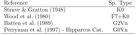
Table 1: Various determinations of the RZ Com spectral type.
Reference Sp. Type
Struve & Gratton (1948) K0
Wood et al. (1980) F7+K0
Batten et al. (1989) G2Vn
Perryman et al. (1997) - Hipparcos Cat. G0Vn
Rovithis-Livaniou et al. (2002) also published a paper attempting to analyze the period variations; however the listed data—while numerous—did not allow for any meaningful conclusions about the period behaviour due to the limited time interval spanned by the data. In addition, they did point to the lack of agreement as to the spectral type, refer-encing four disparate classifications. These are given in Table 1.
Xiang & Zhou (2004) obtained aB band light curve at the Yunan Observatory in China
using the 1.00-m reflector telescope and a CCD camera. They extracted five new times of minima from their published data and proceeded to perform a photometric analysis using the 1992 version of the Wilson-Devinney code. Using the ’q-search’ method they obtained two solution sets with mass ratio values of 0.8 and 2.2 and “[could not] say which of the two results is accurate”. This is in spite of the fact that there were two radial velocity datasets available Struve & Gratton (1948); McLean & Hilditch, (1983) which would have resolved the issue. Unfortunately, there also seemed to be some confusion between
the different naming conventions (for m1 and m2) typically used by spectroscopists and
photometrists.
Lastly, Qian (2001) and Qian & He (2005) presented period analyses. The latter paper presented four new times of minima and a light time effect (LiTE) analysis of the—by now—extensive data set. The analysis was updated in a review paper by Nelson et al. (2016), who obtained similar results. Both LiTE fitting results, along with those of this paper, are presented in Table 14.
Because more modern techniques promised to improve the radial velocity data, the lead author (R.H.N.) first secured, in the springs of 2016, 2017, and 2018, a total of 14
medium resolution (R∼10000 on average) spectra of RZ Com at the DAO using the 1.83
m Plaskett Telescope. This system features a Cassegrain spectrograph fitted with (in
this case) the 21181Yb grating (1800 lines/mm and blazed at 5000 ˚A) which produces a
first order linear dispersion of 10 ˚A/mm. The wavelengths ranged from 5000 to 5260 ˚A,
approximately. A log of observations is given in Table 2 and an eclipse timing diagram, in Figs. 11 and 12 later in the paper. The latter was used to derive the following elements (Eq 1), used for both this photometric data set and also RV phasing:
JD (Hel) Min I = 2458253.6296 (152) + 0.3385075 (4) (1)
where the quantities in brackets are the standard errors of the preceding quantities in units of the last digit.
Frame reduction was performed by software RaVeRe (Nelson 2013). See Nelson
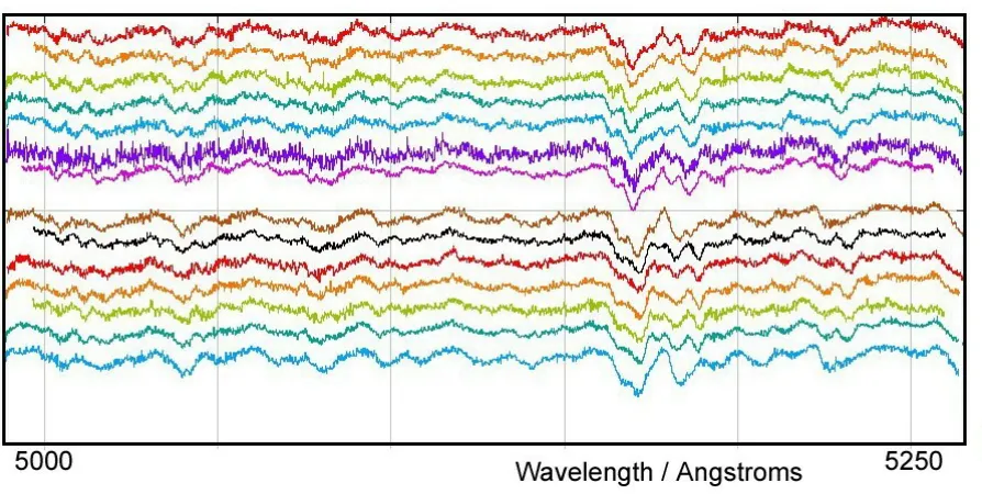
(2010) and Nelson et al. (2014) for further details. The normalized spectra are reproduced in Fig. 1, sorted by phase (the vertical scale is arbitrary). Note towards the right the strong
neutral iron lines (at 5167.487 and 5171.595 ˚A) and the strong neutral magnesium triplet
(at 5167.33, 5172.68, and 5183.61 ˚A).
Radial velocities were determined using the Rucinski broadening functions (Rucinski
Table 2: Log of DAO observations.
DAO Mid Time Exposure Phase at V1 V2
Image # (HJD−2400000) (sec) Mid-exp (km/s) (km/s)
16-1275 57493.7798 2831 0.294 −228.7 (4.9) 133.0 (5.1)
16-1331 57495.9583 3600 0.729 254.1 (2.2) −94.3 (6.1)
16-1431 57498.6938 3600 0.810 241.6 (2.6) −89.2 (4.5)
16-1433 57498.7365 3600 0.937 — −33.0 (2.6)
16-1439 57498.8335 3600 0.223 −232.8 (4.0) 123.4 (4.1)
16.1441 57498.8774 3600 0.353 −173.1 (2.5) 85.3 (2.3)
16-1455 57499.6844 2400 0.737 270.4 (3.0) −103.5 (3.2)
16-1467 57500.8635 1605 0.220 −235.2 (3.7) 122.4 (4.9)
16-1484 57504.7129 2100 0.592 136.6 (7.1) −81.4 (4.5)
16-1502 57504.9060 1800 0.162 −203.0 (4.6) 103.4 (3.5)
17-3989 57859.7304 900 0.365 −177.9 (4.9) 116.7 (3.1)
18-5239 58231.8677 1800 0.712 258.7 (3.2) −102.1 (5.5)
18-5342 58233.9179 1800 0.769 268.7 (2.3) −101.7 (6.7)
18-5486 58241.8496 1800 0.200 −222.4 (3.9) 114.5 (2.0)
Figure 1. RZ Com spectra at phases 0.162, 0.200, 0.220, 0.223, 0.294, 0.353, 0.365, 0.592, 0.712, 0.729, 0.737, 0.769, 0.810, 0.937 (from top to bottom). Each has been shifted vertically for clarity. The
[image:4.595.78.525.450.675.2]et al. (2014) for further details. An Excel worksheet (with built-in macros written by him) was used to do the necessary radial velocity conversions to geocentric and back to heliocentric values (Nelson 2014). The resulting RV determinations are also presented in Table 2 along with standard errors (in units of the last digits, enclosed in brackets). The
mean rms errors for RV1 and RV2 are 6.9 and 11.7 km/s, respectively, and the overall rms
deviation from the (sinusoidal) curves of best fit is 12.6 km/s. The best fit yielded the values K1 = 249.5(0.7) km/s, K2 = 114.9(0.9) km/s and Vγ = 11.5(0.5) km/s, and thus a
mass ratio qsp =K1/K2 =m2/m1 = 2.17(2).
[image:5.595.86.512.257.426.2]Representative broadening functions, at phases 0.223 and 0.737 are depicted in Figs. 2 and 3, respectively (the vertical scale is arbitrary). Smoothing by a Gaussian filter is routinely done in order to centroid the peak values for determining the radial velocities.
[image:5.595.86.514.506.675.2]Figure 2. Broadening functions (arbitrary intensity) at phase 0.223—smoothed and unsmoothed.
Figure 3. Broadening functions (arbitrary intensity) at phase 0.223—smoothed and unsmoothed.
During four nights in 2018, May 8-18, the lead author took a total of 164 frames inV,
168 in RC (Cousins) and 165 in the IC (Cousins) bands at Desert Blooms Observatory,
Table 3: Details of variable, comparison and check stars.
Object TYC RA (J2000) Dec (J2000) V (mag) B−V (mag)
Variable 1990-2841-1 12h35m05.06s +23◦
20′
14′′.
0 10.440 (32) +0.506 (49)
Comparison 1990-1707-1 12h34m24.41s +23◦
27′
14′′.
4 10.571 (57) 0.415 (60)
Check 1990-3503-1 12h35m18.50s +23◦
18′
11′′.
4 12.161 (48) 0.537 (56)
near Benson Arizona, the telescope is operated remotely. It consists of a Software Bisque Taurus 400 equatorial fork mount, a Meade LX-200 40 cm Schmidt-Cassegrain optical
assembly operating at f/7, a SBIG STT-1603 XME CCD camera (with a field of view 11×
18′
), and a filter wheel with the usualB,V,RC, andIC filters. For unattended operation, automatic focusing is required owing to the large temperature changes throughout the night (typically +35◦
to +10◦
C in late spring).
Standard reductions were then applied (see Nelson et al. 2014 for more details). The variable, comparison, and check stars are listed in Table 3. The coordinates are from the Gaia Catalogue, DR2 and magnitudes are from the APASS catalogue DR9 (Henden, et al. 2009, 2010; Smith et al. 2010).
Radial velocity and light curve analysis was carried out using the 2003 version of the Wilson-Devinney (WD) analysis program with Kurucz atmospheres (Wilson & Devinney, 1971, Wilson et al. 1972, Kurucz 1979, Wilson 1990, Kallrath & Milone 1998, Wilson
1998) as implemented in the Windows front-end software WDwint Nelson (2013). In
this process, the first task one faces is to determine the effective temperature of the more luminous component, either from the published spectral type or by some other means. However, as noted in Table 1, the correct classification is unclear. Following the initial classification of Struve & Gratton (1948), which was from actual spectra, and also that of earlier workers, the lead author initiated modelling assuming a spectral type of K0
and an effective temperature T2 of 5247 ± 150 K based on the calibration of Flower
(1996). The choice of this later spectral type was further justified because the computed
total mass from the RV curves (assuming 90◦
inclination) was 1.70 solar masses which nicely corresponds to the tabular value of 1.60 solar masses for a main-sequence G9+K0 pair. Also, because the system was known to be of the W-type subclass (the secondary star in this convention) is the more massive, and can be expected to be more luminous,
therefore dominating the classification spectra. Therefore temperature T2 was held fixed,
and temperature T1 was varied to attain the best fit. (In view of the ‘approximate’
characterization of Struve & Gratton’s classification, the error estimate forT2 is based on
112 subclasses.) From the interpolated tables of Cox (2000), a logg value of 4.476 (cgs) was assumed.
An interpolation program by Terrell (1994), available from Nelson (2013) gave the Van Hamme (1993) limb darkening values; and finally, a logarithmic (LD=2) law for the limb
darkening coefficients was selected, appropriate for temperatures < 8500 K (ibid.). The
limb darkening coefficients are listed below in Table 4. The values for the second star are
based on the later-determined temperature of T1 = 5420 K, logg1 = 4.475 (and assumed
spectral type of G8.) Convective envelopes for both stars were used, appropriate for cooler stars (hence values gravity exponent g = 0.32 and albedoA= 0.5 were used for each).
From the GCVS 4 designation (EW/KW) and from the shape of the light curve, mode 3 (overcontact) mode was used. Initial fitting was accomplished in LC mode by examining
the computed and actual light curves in one passband (V), and adjusting the parameters.
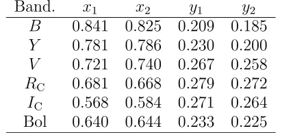
Table 4: Limb darkening values from Van Hamme (1993) forT1,2 and logg1,2as above. The Y band was used in Broglia (1960) and corresponds to a central wavelength of 5300 Angstroms.
Band x1 x2 y1 y2
B 0.849 0.851 0.078 0.040
Y 0.795 0.802 0.166 0.150
V 0.782 0.790 0.187 0.156
RC 0.713 0.725 0.220 0.198
IC 0.628 0.638 0.223 0.207
Bol 0.648 0.647 0.188 0.175
Kallrath & Milone (1998) for an explanation of the method.) The subsets were: (a, Vγ,
q, L1), (T1, Ω1), and (i, L1). Following the recommendation of Binnendijk (1964), a cool
spot was added to star 2 near the neck (that is, with a longitude near 0◦
). At the time, it was believed necessary to add third light, l3.
Following the example of Alton (2010) in which a unified physical light curve model for AC Boo was achieved for no fewer than eight data sets (the light curve differences being due to a time-varying cool spot), the lead author (RHN) proceeded to attempt the same feat using the data sets of Broglia (1960), Xiang & Zhou (2004), Rovithis & Rovithis-Livaniou (1984), and He & Qian (2008). No solution for the third (R&R-L) data set was possible owing to the strange, non-standard shape of the light curves, and to the disparate eclipse depths between light curves. The eclipse depths were compara-ble in the blue bandpass while, in the visual bandpass, the secondary depth was much shallower. (No known mechanism could account for this disparity, so modelling attempts were abandoned.)
However, comparable fits were achieved for the present data set, and for those of the other three listed above. All spots were placed on star 2 (the more massive) with the exception of the data of Xiang & Zhou (2004), for which the best solution involved no spot. However, there was a snag. When the co-author (KBA) joined the study, he pointed
out that, based on his compilation of contemporary colour magnitude differences (B−V),
the system was likely hotter. Further, the Tycho catalogue Wright, et al., (2003) lists the
system as G0Vn, temperature T2 = 6030 K, logg2 = 4.371. (It was later determined that
T1 = 6236 K and logg1 = 4.365).
No definitive stellar classification supported by UV or-visible spectra is published for
RZ Com. Instead, we relied upon an ensemble ofB −V colour indices from astrometric
and photometric catalogues available through VizieR and those published by Terrell et al. (2012). (See Table 5.) Colour excess was estimated according to Amˆores & L´epine (2005) using the companion program ALextin which requires the Galactic coordinates (l,b) and an estimated distance in kpc. The most recent parallax values reported in Gaia DR2 were used (Gaia Collaboration, 2018). Accordingly Alextin iterated a value for interstellar extinction AV, (which led to the corresponding dereddeningE(B−V) =AV/3.1 correction
for objects within the Milky Way Galaxy and ultimately intrinsic colour (B − V)0).
Outliers within the different sources used for B − V colour indices were statistically
eliminated from consideration using Grubbs Test (Grubbs 1950) as implemented in the
Real Statistics package for Excel. Thereafter the median (B −V)0 result was used to
define the effective temperature of the more luminous star and its corresponding spectral class Pecaut & Mamajek (2013). When we used this approach, the adopted effective
temperature (Teff2 = 6070 K) for RZ Com (Table 5) proved to be slightly higher (6070 vs.
Table 5: Spectral classification of RZ Com based upon dereddeneda
(B−V) data from various catalogues and surveys.
Catalogue/Survey (B −V)0 Teff2b Spectral ClassC
Tycho 0.5100 6240 F7V-F8V
2MASS 0.5539 6034 F9V-G0V
SDSS-DR9 0.5154 6216 F7V-F8V
Terrell et al. (2012) 0.5456 6072 F8V-F9V
APASS 0.4996 6280 F6V-F7V
ASCC 0.5506 6047 F8V-F9V
a:E(B−V) = 0.0074;
b:Teff2 interpolated + spectral class assigned for most luminous star from Pecaut & Mamajek (2013); c: Median value for (B−V)0 = 0.546±0.008; Teff2= 6070±93 K; Spectral class = F8V-F9V
Table 6: New times of minima for V500 Cyg obtained in this study.
Band. x1 x2 y1 y2
B 0.841 0.825 0.209 0.185
Y 0.781 0.786 0.230 0.200
V 0.721 0.740 0.267 0.258
RC 0.681 0.668 0.279 0.272
IC 0.568 0.584 0.271 0.264
Bol 0.640 0.644 0.233 0.225
parameters (Andrae et al. 2018).
It could be argued that the orbital phase at which each of the above (B−V)0
obser-vations was taken is unknown, and therefore taking the mean is questionable. However, in view of the fact that the temperatures of each component are shown below to be very close, it is unlikely that the colour indices could vary to any great extent over an orbital cycle, and certainly less than the variations between values displayed above.
Accordingly, revised values from the van Hamme tables for T1,2 = 6276, 6070 K,
logg1,2 = 4.365, 4.371 respectively were determined and listed in Table 6.
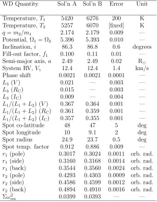
We will start with the 2018 data sets presented in this paper; the two solutions are presented in Table 7. Owing to the fact that the light curve plots are virtually indistin-guishable, only one plot (B) is presented in Fig. 4.
From Mochnacki (1981), the fill-out factor is f = (ΩI−Ω)/(ΩI−ΩO), where Ω is the
modified Kopal potential of the system, ΩI is that of the inner Lagrangian surface, and
ΩO, that of the outer Lagrangian surface, was also calculated.
For the most part, the error estimates (for this data set only) are those provided by the WD routines and are known to be underestimated; however, it is a common practice to quote these values and we do so here. Also, estimating the uncertainties in temperatures
T1 and T2 is somewhat problematic. A common practice is to quote the temperature
difference over–say–one spectral sub-class. assuming that the classification is good to one spectral sub-class, (the precision being unknown in this case). In addition, various different calibrations have been made Flower (1996) and Pecaut & Mamajek (2013), and
classification is ± one sub-class, an uncertainty of± 200 K to the absolute temperatures
of each, would be reasonable. (The modelling error in temperature T1, relative to T2, is
indicated by the WD output to be much smaller, around 9 K.)
Trials were also run with the spot on the neck side of star 1 (the hotter star); however,
[image:8.595.196.410.291.388.2]Table 7: Wilson-Devinney parameters for the present dataset.
WD Quantity Sol’n A Sol’n B Error Unit
Temperature, T1 5420 6276 200 K
Temperature, T2 5257 6070 [fixed] K
q=m2/m1 2.174 2.179 0.009 —
Potential, Ω1 = Ω2 5.396 5.393 0.010 —
Inclination, i 86.3 86.8 0.6 degrees
Fill-out factor, f1 0.100 0.11 0.01 —
Semi-major axis, a 2.49 2.49 0.02 R⊙
System RV, Vγ 12.4 12.4 1.4 km/s
Phase shift 0.0021 0.0021 0.0001 —
L3 (V) 0.021 — 0.003 —
L3 (RC) 0.015 — 0.003 —
L3 (IC) 0.009 — 0.004 —
L1/(L1+L2) (V) 0.367 0.364 0.001 —
L1/(L1+L2) (RC) 0.361 0.359 0.001 —
L1/(L1+L2) (IC) 0.357 0.355 0.001 —
Spot co-latitude 48 47 5 deg
Spot longitude 10 9.1 2 deg
Spot radius 24.9 23.7 0.5 deg
Spot temp. factor 0.912 0.886 0.009 —
r1 (pole) 0.3017 0.3024 0.0011 orb. rad.
r1 (side) 0.3160 0.3168 0.0014 orb. rad.
r1 (back) 0.3544 0.3560 0.0024 orb. rad.
r2 (pole) 0.4293 0.4303 0.0009 orb. rad.
r2 (side) 0.4586 0.4599 0.0012 orb. rad.
r2 (back) 0.4894 0.4910 0.0016 orb. rad.
Σω2
6070 K) further trials were run with third light, however they did not improve the fit. An effort was made to go back to test the idea that solution A could be improved by deleting third light. A number of trials were run with no success. In view of the fact that solution
B (T2 = 6070 K) of is considered to be the optimum solution, there seemed to be no point
in pursuing the matter further. The question then arises as to why we include Solution A at all. The answer is that it can serve as a cautionary tale to modellers in that different parameters can lead to nearly identical residuals and identical plots. In the case of AR CrB, this effect is illustrated more rigorously after adjusting the effective temperature of
the more luminous star by as much as 3σ (Alton & Nelson 2018). It is the task of the
modeller to sort out the best values based on external criteria.
The light curve data and the fitted curves from this paper are depicted in Fig. 4 (from
top to bottom: V, RC, and IC), shifted by 0.1 flux units. The residuals in the sense
[image:10.595.89.517.299.496.2](observed-calculated) are also plotted, shifted downward, and from each other by 0.05 units.
Figure 4. (top to bottom)V, RC, andIClight curves for RZ Com (this paper) – Data, WD fit,
residuals. For clarity, the top three curves were offset by 0.10 divisions, while the bottom three, by 0.05 divisions.
Next, the data sets from Broglia (1960) were modelled, starting with data set 1. The solutions from this paper, along with those in Wilson & Devinney (1973), are presented in Table 8.
Next, the second dataset from Broglia (1960) was modelled. The solutions from this paper, along with those in Wilson & Devinney (1973), are presented in Table 9.
This time, the plots for both data sets are combined and presented in Fig. 5. Once again, plots for the two solutions are indistinguishable; hence only one figure is required.
Table 8: Wilson-Devinney parameters for the first dataset of Broglia (1960).
WD Quantity. W&D 1973 Sol’n A Sol’n B Error Unit
Temperature, T1 5500 5420 6307 19 K
Temperature, T2 5564 5257 6070 [fixed] K
q =m2/m1 2.292 (30) 2.185 2.22 0.02 —
Potential, Ω1 = Ω2 5.618 (54) 5.396 5.44 0.03 —
Inclination, i 86.04 (51) 85.7 86.0 1.1 deg.
Fill-out factor, f1 0.042 0.12 0.15 0.02 —
Semi-major axis, a na 2.49 2.48 0.02 R⊙
System RV, Vγ na 12.4 12.2 1.2 km/s
Phase shift — 0.0006 0.0006 0.0004 —
L3 (Y) — 0.015 — — —
L1/(L1+L2) (Y) na 0.366 0.366 — —
Spot co-latitude — 76 80 10 deg
Spot longitude — 4 3.5 8 deg
Spot radius — 27 26.6 4 deg
Spot temp. factor — 0.9596 0.946 0.016 —
r1 (pole) 0.2924 (44) 0.3026 0.3023 0.0026 orb. rad.
r1 (side) 0.3056 (52) 0.3172 0.3169 0.0033 orb. rad.
r1 (back) 0.3403 (82) 0.3567 0.3573 0.0058 orb. rad.
r2 (pole) 0.4287 4(2) 0.4310 0.4333 0.0022 orb. rad.
r2 (side) 0.4574 (55) 0.4608 0.4636 0.0029 orb. rad.
r2 (back) 0.4859 (71) 0.4921 0.4952 0.0040 orb. rad.
Σω2
res — 0.0046 0.0046 — —
Table 9: Wilson-Devinney parameters for the second dataset of Broglia (1960).
WD Quantity.. W&D 1973 Sol’n A Sol’n B Error Unit
Temperature, T1 5500 5470 6325 14 K
Temperature, T2 5552 5257 6070 [fixed] K
q =m2/m1 2.394 (20) 2.19 2.20 0.04 —
Potential, Ω1 = Ω2 5.869 (40) 5.40 5.40 0.09 —
Inclination, i 85.72 (31) 86.3 86.3 0.6 degrees
Fill-out factor, f1 -0.059 0.12 0.13 0.03 —
Semi-major axis, a na 2.49 2.49 0.02 R⊙
System RV, Vγ na 12.4 12.4 1.1 km/s
Phase shift — 0.0001 0.0001 0.0003 —
L3 (Y) — 0.013 — — —
L1/(L1+L2) (Y) na 0.376 0.377 — —
Spot co-latitude — 115 115 10 deg
Spot longitude — 0 0 8 deg
Spot radius — 27.0 27 4 deg
Spot temp. factor — 0.971 0.971 0.016 —
r1 (pole) 0.2805 (30) 0.3030 0.3038 0.0083 orb. rad.
r1 (side) 0.2918 (35) 0.3177 0.3186 0.0101 orb. rad.
r1 (back) 0.3211 (52) 0.3577 0.3596 0.0176 orb. rad.
r2 (pole) 0.4240 (29) 0.4317 0.4331 0.0074 orb. rad.
r2 (side) 0.4509 (37) 0.4617 0.4635 0.0098 orb. rad.
r2 (back) 0.4761 (47) 0.4933 0.4955 0.0132 orb. rad.
Σω2
[image:11.595.115.488.451.777.2]Figure 5. Y light curves (1 & 2) of Broglia (1960) – Data, our WD fits, residuals. For clarity, the curves have been offset as in Fig. 4.
The two solutions from this paper, along with those from Xiang & Zhou (2004), are presented in Table 10.
This time, there is a significant difference in the plots for solutions A & B; hence both are presented, in Figs. 6 and 7.
Figure 6. B light curve of Xiang & Zhou (2004): – Data, our WD fit A, (residuals offset)
And, lastly, we modelled the data of He & Qian (2008). As the analysis occurred late in the paper writing, we did not attempt a fit using the lower temperatures, but merely started with the parameters obtained from the other datasets. To our surprise, the spot had moved significantly in longitude. The results are listed in Table 11.
The light curve data from He & Qian (2008) and the fitted curves from this paper
[image:12.595.85.515.429.628.2]Table 10: Wilson-Devinney parameters for the dataset of Xiang & Zhou (2004).
WD Quantity... Xiang & Zhou Tbl 5 Xiang & Zhou Tbl 6 Sol’n A Sol’n B Error Unit
Temperature, T1 4900 4900 5425 6289 18 K
Temperature, T2 4842 4802 (9) 5257 6070 [fixed] K
q=m2/m1 2.226 (13) 0.772 (9) 2.19 2.20 0.02 — Potential, Ω1 = Ω2 5.267 (15) 3.330 (14) 5.39 5.40 0.02 — Inclination,i 79.67 (28) 78.40 (31) 83.2 81.6 0.5 degrees Fill-out factor, f1 na na 0.13 0.12 0.01 —
Semi-major axis, a na na 2.49 2.51 0.02 R⊙
System RV,Vγ na na 12.4 12.2 1.1 km/s
Phase shift na na -0.0056 -0.0055 0.0005 —
L3 (B) — — 0.053 — — —
L1/(L1+L2) (B) 0.3699 (31) 0.3833 (11) 0.378 0.376 0.002 —
r1(pole) 0.3090 (8) 0.4051 (14) 0.3039 0.3039 0.0027 orb. rad.
r1(side) 0.3246 (10) 0.4376 (17) 0.3187 0.3188 0.0034 orb. rad.
r1(back) 0.3676 (17) 0.4376 (17) 0.3595 0.3599 0.0062 orb. rad.
r2(pole) 0.4327 (17) 0.3403 (34) 0.4327 0.4334 0.0018 orb. rad.
r2(side) 0.4634 (23) 0.3573 (43) 0.4630 0.4639 0.0025 orb. rad.
r2(back) 0.4967 (33) 0.3921 (69) 0.4949 0.4960 0.0036 orb. rad. Σω2
res 0.003617 0.004221 0.0091 0.0088 — —
[image:13.595.93.516.490.682.2]Table 11: Wilson-Devinney parameters for the dataset of He & Qian (2008).
WD Quantity.... He & Qian 2008 Our sol’n Error Unit
Temperature, T1 5000 6267 13 K
Temperature, T2 4900 (8) 6070 — K
q=m2/m1 2.351 (31) 2.174 0.062 —
Potential, Ω1 = Ω2 5.620 (45) 5.38 0.19 —
Inclination, i 81.4 (4) 84.9 0.4 degrees
Fill-out factor, f1 0.201 (74) 0.11 0.01 —
Semi-major axis, a — 2.49 0.03 R⊙
System RV, Vγ — 12.4 1.8 km/s
Phase shift — -0.0005 0.0003 —
L1/(L1 +L2) (B) 0.3471 (37) — — —
L1/(L1 +L2) (V) 0.3545 (41) 0.364 0.001 —
r1 (pole) 0.2971 (45) 0.3026 0.0177 orb. rad.
r1 (side) 0.3113 (55) 0.3171 0.0215 orb. rad.
r1 (back) 0.3512 (98) 0.3664 0.0362 orb. rad.
r2 (pole) 0.4371 (37) 0.4302 0.0163 orb. rad.
r2 (side) 0.4682 (49) 0.4598 0.0215 orb. rad.
r2 (back) 0.4990 (67) 0.4910 0.0287 orb. rad.
Σω2
res 0.00101 0.0235 — —
residuals in the sense (observed-calculated) are also plotted, shifted downward, and from each other by 0.05 units.
The radial velocities are plotted in Fig. 9. Three-dimensional representations created using Binary Maker 3 (Bradstreet, 1993) for each of the studied epochs are shown in Fig. 10. (The crosses represent the centres of mass of the individual stars and of the system as a whole.)
From the WD output parameters we calculated the fundamental properties
correspond-ing to each of the T2 = 6070 K solutions; the results are listed in Table 12. Most of the
errors are output or derived estimates from the WD routines. The values from Hilditch et al. (1988) as reported in Yildiz & Do˘gan (2013; hereafter Y&D) are included in column 2 for comparison.
Also included for comparison in Table 12 are the interpolated values from Pecaut & Mamajek (2013) for single main-sequence stars (as a function of temperature), in column 8. As noted in Y&D, the values for the more massive starm2 (in our convention) are not far off the main sequence values. On the other hand, the less massive star is either under-luminous for a star of its temperature (and therefore spectral class), or is over-under-luminous for a main sequence star of the same mass. From the interpolated tables of Pecaut &
Mamajek (2013), the primary of mass 0.57 M⊙ should have a luminosity of 0.093 L⊙. See
the concluding remarks for more discussion on this point.
To determine the distances rfor the present data in the last row, we proceeded as
fol-lows: First the WD routine gave the absolute bolometric magnitudes of each component; these were then converted to the absolute visual (V) magnitudes of both,MV,1 and MV,2,
using the bolometric corrections BC =−0.06 and−0.08 for stars 1 and 2 respectively. The latter were taken from tables constructed from Pecaut & Mamajek (2013). The absolute
Figure 8. B andV light curves of He & Qian (2008) – Data, our WD fits, residuals. For clarity, the curves have been offset as in Fig. 4.
[image:15.595.86.513.494.693.2]Figure 10. Binary Maker 3 representations of the system. Top to bottom: Broglia (1960) data set 1, Broglia (1960) data set 2, Xiang & Zhou (2004), He & Qian (2008), dataset from this paper (2018).
Table 12: Fundamental parameters. Errors are for the data set of this paper only.
Quantity Hilditch Broglia Broglia Xiang- He & This Error Cox unit (1988) 1 2 Zhou Qian dataset (2000) unit Temp.,T1 6457 (298) 6307 6325 6289 6267 6246 200 — K Temp.,T2 6166 (284) 6070 6070 6070 6070 6070 [fixed] — K Mass,m1 0.55 (4) 0.557 0.570 0.582 0.574 0.573 0.007 1.55 M⊙ Mass,m2 1.23 (9) 1.239 1.253 1.282 1.248 1.249 0.009 1.16 M⊙ Radius,R1 0.78 (2) 0.81 0.82 0.83 0.82 0.82 0.01 1.22 R⊙ Radius,R2 1.12 (3) 1.16 1.16 1.17 1.15 1.15 0.01 1.11 R⊙
Mbol,1 — 4.86 4.82 4.83 4.87 4.87 0.01 3.77 mag
Mbol,2 — 4.26 4.25 4.41 4.26 4.26 0.01 4.12 mag
logg1 — 4.36 4.36 4.37 4.37 4.37 0.01 4.36 cgs logg2 — 4.40 4.41 4.41 4.41 4.41 0.01 4.37 cgs Luminosity,L1 0.93 (15) 0.94 0.97 0.96 0.93 0.93 0.03 2.04 L⊙ Luminosity,L2 1.62 (26) 1.63 1.64 1.68 1.63 1.63 0.03 1.16 L⊙
Distance,r — 204 204 204 201 204 5 — pc
The apparent magnitude in theV passband wasV = 10.44±0.03, taken from the APASS
catalogue (Henden et al., 2009, 2010; Smith et al. 2010). In order to check that the values were obtained at the correct phase (i.e., near phase 0.25 or 0.75—when the flux from both stars was maximum), photometry at these phases was analysed using the comparison star
and its V magnitude of 10.571 (57), also taken from the APASS catalogue. The result:
V = 10.437 (5) where the error stated is the standard error of the mean; including the
error in the comparison magnitude, resulted in V = 10.44 (6).
Because of the system’s high galactic latitude (+84.7◦
), and as we will see, its close proximity, interstellar absorption, AV may be ignored initially. Therefore using the
stan-dard relation (Eq 2) with AV = 0, we calculated a value for the distance as r= 209 pc:
r = 100.2(V−M v−AV+5) parcsec (2)
Galactic extinction was obtained from a model by Amˆores & L´epine (2005). The code available in IDL (and converted by the author to a Visual Basic routine) assumes that the interstellar dust is well mixed with the dust, that the galaxy is axi-symmetric, that the gas density in the disk is a function of the Galactic radius and of the distance from the Galactic plane, and that extinction is proportional to the column density of the gas, Using Galactic coordinates ofl = 257.7516◦
andb = +84.7047◦
(SIMBAD), and the initial
distance estimate of d = 0.208 kpc, a value of AV = 0.070 magnitude was determined.
A further iteration revealed little change in AV. Substitution into (2) gave r = 202 pc.
Similar calculations were carried out for the other datasets.
However, there was a problem. The value derived from the Schlegel dust maps (Schlegel et al. 1998)1, and including the factor sin(galactic latitude) is A
V = 0.045 mag. As
this value pertains to the absorption all the way through the Galactic arm (a distance of approximately 0.3 kpc), the value from Amˆores & L´epine appears to overestimate interstellar extinction in this region of the sky. If we take 2/3 of the Schlegel value (2/3×0.045) we getAV = 0.03 mag. Substitution into (2) gave r = 206 pc, close to the
above value. Therefore we adopt the mean of the two computed values, 204 pc. The same procedure was used with the other datasets in Table 12.
The errors were assigned as follows: δMbol,1 =δMbol,2 = 0.02, δBC1 =δBC2 = 0.005
(the variation of 1/2 spectral sub-class), δV = 0.04, all in magnitudes. Combining the
errors rigorously (i.e., by adding the variances) yielded an estimated error in r of 5 pc.
1available at:
Table 13: New times of minima for RZ Com obtained in this study.
Min (Hel)−2400000 Type Error (days)
58169.8508 II 0.0002
58246.8611 I 0.0004
58250.7519 II 0.0002
58253.7986 II 0.0002
Table 14: LiTE parameters from various sources.
LiTE Quantity Qian &He 2005 He & Qian 2008 Nelson et al. 2016 This work Unit Period,P3 44.8 (7) 45.1 (6) 41.4 (5) 41.4 (7) years Amplitude,A 0.0058 (5) 0.0065 (1) 0.0063 (3) 0.0063 (4) days Eccentricity,e3 0 0 0.30 (11) 0.30 (12) — Arg. Periastr.,ω3 260 (7) 278 (7)- 472 (25) 472 (35) degrees Periastron time — — 42744 (1790) 42772 (2643) HJD−2400000
a12 sini 1.00 (9) 1.12 (2) 1.09 (6) 1.10 (6) AU
f (m3) 0.00051 (13) — 0.00076 (12) 0.00077 (14) M⊙
dP/dt(1-2 pair) 4.12 3.97 3.86 (8) 3.84 (2) 10-8 d/yr
The Gaia DR2 catalogue lists, for RZ Com, a parallax of 4.898±0.088 mas. This
translates to a distance of 203.1±3.7 pc, consistent with all our distance estimates. Four new times of minima emerged from the observations; these are reported in Table 13. Each is the mean of three values (one for each filter). For each filter, five methods of minimum determination, as implemented in software Minima23 Nelson (2013) were used: the digital tracing paper method, bisection of chords, sliding integrations (Ghedini 1982), curve fitting using five Fourier terms, and Kwee and van Woerden (Kwee & Woerden 1956, Ghedini 1982). There was no significant difference between corresponding values for the different filters. Because, in the literature, many (or perhaps most) error estimates can be shown to be low (sometimes unrealistically so), the estimated errors were taken as double the standard deviations of the various determinations. Also, a minimum error value of 0.0002 days was adopted for the same reason.
The period behaviour of this system is very interesting, and was earlier examined in Nelson et al. (2016). An eclipse timing difference (O–C) plot using the same timings dating from 1927 but updated with more recent points was used. Earlier fits are due to Qian & He (2005) and He & Qian (2008). As with Nelson et al. (2016), derivations of the light time effect (LiTE) using relations from Irwin (1952, 1959), resulted in a good fit. Standard weighting was used: pg = 0.2, vis = 0.1, and PE, CCD = 1.0.
As the reader will see in Table 14, parameters in the updated fit differ only slightly (if at all) from Nelson et al. (2016).
The eclipse timing difference (O–C) plot with all available timings together with the latest LiTE fit is depicted in Fig. 11.
From the definition of the mass function given in equation 3:
f(m3) = (m3sini′
)3/(m1+m2+m3)2 (3)
and the value from this work, we were able to estimate a value form3. Assuming that
the inclination i′
of the putative third star orbit is the same as that of the eclipsing pair (viz. 85◦
), we calculated mass m3 by iteration, obtaining the value m3 = 0.144 (8) M⊙.
From the tables of Cox (2000) for main sequence stars, we read that the luminosity would
be 0.0009 L⊙, which is far too faint to be of any consequence to the modelling process
[image:18.595.71.529.204.303.2]Figure 11. RZ Com – eclipse timing (O–C) diagram with LiTE fit (see text). [Note: (green) squares = photographic; (yellow) pyramids = visual; (red) circles = photoelectric; and (black) diamonds = CCD.]
Elements used to generate this plot are given in Equation 4.
JD (Hel) Min I = 2443967.9371 (29) + 0.33850604 (5) E (4)
In order to phase the photometric and radial velocity curves correctly, a different set of elements, applying to the interval over which the data were taken, was required. For the present data set, timings from 2014-2018 were used with the exclusion of all else; the results of the fit are shown in Fig. 12.
This resulted in the elements of Equation 5 given below. These elements were used for all phasing of the RV and present photometric data.
JD (Hel) Min I = 2458253.6296 (29) + 0.3385075 (5) E (5)
Similar fits were used for the other data sets. Elements for the Broglia (1960) photo-metric data were:
JD (Hel) Min I = 2458253.5711 (12) + 0.33850598 (5) E (6)
and those for the Xiang & Zhou (2004) photometric data:
JD (Hel) Min I = 2458253.6628 (29) + 0.3385088 (5) E (7)
Elements were not required for the data of He & Qian (2008) as their reported data were already phased.
Figure 12. RZ Com – eclipse timing (O–C) diagram with LiTE fit (dashed line) and linear fit for the range
Further, once the LiTE fit was achieved, it was now possible to plot the residuals (see Fig. 13); that is the O–C values minus the LiTE component (see Nelson et al. 2016 for details).
The equation of the line of best fit is:
O−C = 0.0078 (8) + 6.6 (1)×10−7
E + 1.79(0.12)×10−11
E2 (8)
From the quadratic coefficient, c2 one calculates the intrinsic rate of period change,
dP/dt by:
dP/dt= 2c2365.24/P = 3.86 (21)×10
−8 days/year (9)
whereP = the orbital period of the eclipsing pair.
If this (constant) rate of period change is due to conservative mass exchange, we may calculate this rate by (see Nelson et al. 2016 for references):
dm1/dt= [3P(1/m2−1/m1)]
−1dP/dt (10)
Substituting the mean stellar masses for m1 and m2 from Table 12, we obtained the
value dm1/dt=−4.1 (3)×10−8 M
⊙/year which means that (as is often the case) the less
massive star is losing mass to its companion.
However, it is not clear that the condition of conservative mass transfer is valid. Y&D concluded that, for overcontact binaries, only 34 per cent of the mass from the lesser
massive star is transferred to the more massive one. Hence, the value for dm1/dt should
be treated with caution. See also Yildiz (2014).
Figure 13. The O–C values for RZ Com minus the LiTE component with the quadratic of best fit.
With our values for the fill-out factor ranging from 0.10 to 0.13, that makes the system a slightly-overcontact binary, typical of the W-types (Rucinski 1974, Kallrath & Milone 1998). Further, our reciprocal mass ratio q′
=m1/m2 = 1/q = 0.45 lies in the middle of the ’moderate’ range (0.4< q′
<0.6), typical of the W-type (Kallrath & Milone 1998). We also found unified solutions for all the datasets (except as noted) spanning some 60 years. A cool spot on the more massive star accounted for the changes in the light curves over time, giving plausible spot configurations. There appears to be an easy progression between the two data sets of Broglia, and also between the datasets of He & Qian, and with ours. There seemed to be no spot at the epoch of the Xiang & Zhou dataset, however, the higher scatter in their dataset does not allow one to be sure. RZ Com is probably a good candidate for extensive coverage in order to map in detail the progression of the spot.
From Table 12, it is evident that star 1 is underluminous compared to a main sequence star of the same temperature or spectral type, or that it is undermassive for its spectral type the two conditions are equivalent (because a less massive star would have a smaller radius, a smaller emitting area, and hence a lower luminosity). This discrepancy was also noted in Wilson & Devinney (1973) who found ‘masses which seem incompatible with their position on the H-R diagram’. However, there is an explanation. According to the calculations of Y&D, the initial mass of the hotter star of RZ Com (designated the
primary here, the secondary in Y&D), was much higher, starting at 1.58 M⊙ followed by
a period of mass exchange, ending up with a mass of 0.55 M⊙, not far from our value of
0.573(7) M⊙. Again, according to Y&D, the luminosity of our primary (m1) would depend
as much on its initial mass as it does on its present mass, hence the excess luminosity [for its mass]. Y&D also determined the main-sequence age to be 2.09 Gyr.
Acknowledgements: It is a pleasure to thank the staff members at the DAO (Dmitry
and assistance. Many thanks are also due to the San Pedro Observatory resident as-tronomer/technician, Dean Salman for his tireless help. Much use was made of the VizieR
search tool along with the SIMBAD and O–C Gateway (B.R.N.O.)2 databases. This
re-search has made use of the APASS database, located at the AAVSO web site. Funding for APASS has been provided by the Robert Martin Ayers Sciences Fund.
References:
Alton, K. B., 2010,JAVSO, 38, 57
Alton, K. B., Nelson, R. H., 2018, MNRAS, 479, 3197 DOI
Amˆores, E. B., L´epine, J. R. D., 2005, AJ,130, 659 DOI
Andrae,R., Fouesneau, M., Creevey, O., et al., 2018,A&A (arXiv: 1804.09374)
Batten A. H., Fletcher J. M., MCarthy D. G., 1989, Publ. DAO, 17
Binnendijk, L., 1964, AJ, 69, 154 DOI
Binnendijk, L., 1970, Vistas in Astronomy, 12, 217 DOI
Bradstreet, D. H., 1993, “Binary Maker 2.0 – An Interactive Graphical Tool for Pre-liminary Light Curve Analysis”, in Milone, E.F. (ed.) Light Curve Modelling of Eclipsing Binary Stars, pp 151-166 (Springer, New York, N.Y.) DOI
Broglia, P., 1960, Contributi Milano-Merate,165
Gaia Collaboration, 2018, A&A, 616, 1 DOI
Cox, A. N., ed., 2000,Allen’s Astrophysical Quantities, 4th ed., (Springer, New York, NY)
DOI
Flower, P. J., 1996, ApJ, 469, 355 DOI
Gaposchkin, S., 1932,VeBB, 9, 1
Gaposchkin, S., 1938,Variable Stars (Harvard Monograph No. 5, Harvard U. Press)
Ghedini, S., 1982, Software for Photometric Astronomy, (Willmann-Bell Inc.)
Grubbs, F. E. 1950, Annals of Mathematical Statistics,21, 27 DOI
He, J.-J., Qian, S.-B., 2008,ChJAA, 8, 465 DOI
Henden, A. A., Welch, D. L., Terrell, D., Levine, S. E. 2009, The AAVSO Photometric
All-Sky Survey, AAS,214, 407.02
Henden, A. A., Terrell, D., Welch, D., Smith, T. C. 2010, New Results from the AAVSO
Photometric All Sky Survey, AAS, 215, 470.11
Hilditch R. W., King D. J., McFarlane T. M., 1988, MNRAS, 231, 341 DOI
Irwin, J. B., 1952, ApJ, 116, 211 DOI
Irwin, J. B., 1959, AJ, 64, 149 DOI
Kallrath, J. & Milone, E.F., 1998,Eclipsing Binary Stars–Modeling and Analysis (Springer-Verlag) DOI
Kopal, Z., 1955, AnAp, 18, 379
Kurucz, R. L., 1979,ApJS, 40, 1 DOI
Kwee, K. K., van Woerden, H., 1956, BAN, 12, 327
McLean, B. J., Hilditch, R. W., 1983, MNRAS, 203, 1 DOI
Mochnacki, S. W., 1981, ApJ, 245, 650 DOI
Nelson, R. H., 2010, “Spectroscopy for Eclipsing Binary Analysis” in The Alt-Az Initia-tive, Telescope Mirror & Instrument Developments (Collins Foundation Press, Santa Margarita, CA), R.M. Genet, J.M. Johnson and V. Wallen (eds)
Nelson, R. H., 2013, Software by Bob Nelson,
https://www.variablestarssouth.org/bob-nelson/
2
Nelson, R. H., 2014, Spreadsheets, by Bob Nelson,
https://www.variablestarssouth.org/bob-nelson/
Nelson, R. H., S¸enavci, H. V., Ba¸st¨urk, ¨O, Bahar, E., 2014, NewA, 29, 57 DOI
Nelson, R. H., Terrell, D., Milone, E. F., 2016, NewAR, 70, 1 DOI
Nelson, R. H., 2016, Bob Nelson’s O–C Files,
http://www.aavso.org/bob-nelsons-o-c-files
Pecaut, M. J., Mamajek, E. E. 2013,ApJS, 208, 9 DOI
Perryman, M. A. C. et al. 1997, A&A, 500, 501,
Qian, S.-B., 2001, MNRAS, 328, 635 DOI
Qian, S.-B., He, J.-J., 2005,PASJ, 57, 977 DOI
Rovithis, P., Rovithis-Livaniou, E., 1984,A&AS, 58, 679
Rovithis-Livaniou, E., Rovithis, P., Djura˘sevi´c, G., 2002,IBVS, 5235, 1
Rucinski, S. M., 1974, AcA, 24, 119
Rucinski, S M., 2004, IAUS, 215, 17
Russell, H. N., Merrill, J. E., 1952, “The Determination of the Elements of Eclipsing
Binary Stars”, Contributions from the Princeton University Observatory, 26, 1
Schlegel, D. J., Finkbeiner, D. P., Davis, M., 1998,ApJ, 500, 525 DOI
Smith, T. C., Henden, A., Terrell, D., 2010, AAVSO Photometric All-Sky Survey Imple-mentation at the Dark Ridge Observatory, SAS.
Struve, O., Gratton, L., 1948, ApJ,108, 497 DOI
Terrell, D., Gross, J., Cooney, W. P. Jr., 2012, AJ, 143, 99 DOI
Terrell, D., 1994, Van Hamme Limb Darkening Tables, vers. 1.1.
Van Hamme, W., 1993,AJ,106, 2096 DOI
Wilson, R. E., Devinney, E. J., 1971, ApJ, 166, 605 DOI
Wilson, R. E., Devinney, E. J., 1973, ApJ, 182, 539 DOI
Wilson, R. E., DeLuccia, M. R., Johnston, K., Mango, S. A., 1972, ApJ, 177, 191 DOI
Wilson, R. E., 1990, ApJ, 356, 613 DOI
Wilson, R. E., 1998, Documentation of Eclipsing Binary Computer Model (available from the author)
Wood F. B., Oliver J. P., Florkowski D. R., Ko h R. H., 1980,A Finding List for Observers
of Interacting Binary Stars, Univ. of Pennsylvania Press
Wright, C. O., et al., 2003, AJ, 125, 359 DOI
Xiang, F. Y. and Zhou, Y. C., 2004, NewA, 9, 273 DOI
Yildiz, M., Do˘gan, T., 2013, MNRAS, 430, 2029 DOI